Equations with large powers. Methodical development in algebra (grade 10) on the topic: Equations of higher degrees

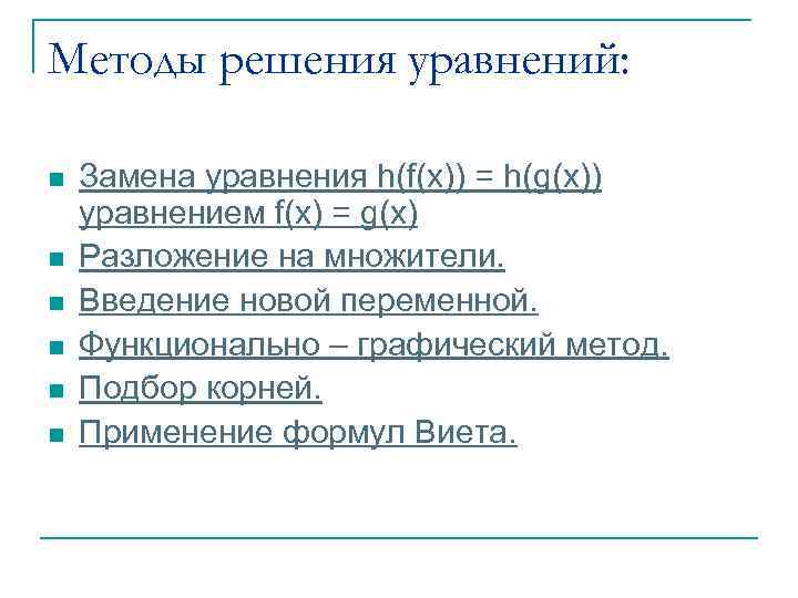Methods for solving equations: n n n Replacing the equation h (f (x)) = h (g (x)) by the equation f (x) = g (x) Factoring. Introducing a new variable. Functionally - graphical method. Selection of roots. Application of Vieta formulas.

Replacing the equation h (f (x)) = h (g (x)) by the equation f (x) = g (x). The method can be used only in the case when y = h (x) is a monotonic function that takes each of its values once. If the function is non-monotonic, then the loss of roots is possible.

Solve the equation (3 x + 2) ²³ = (5 x - 9) ²³ y = x ²³ an increasing function, therefore from the equation (3 x + 2) ²³ = (5 x - 9) ²³ you can go to the equation 3 x + 2 = 5 x - 9, whence we find x = 5, 5. Answer: 5, 5.

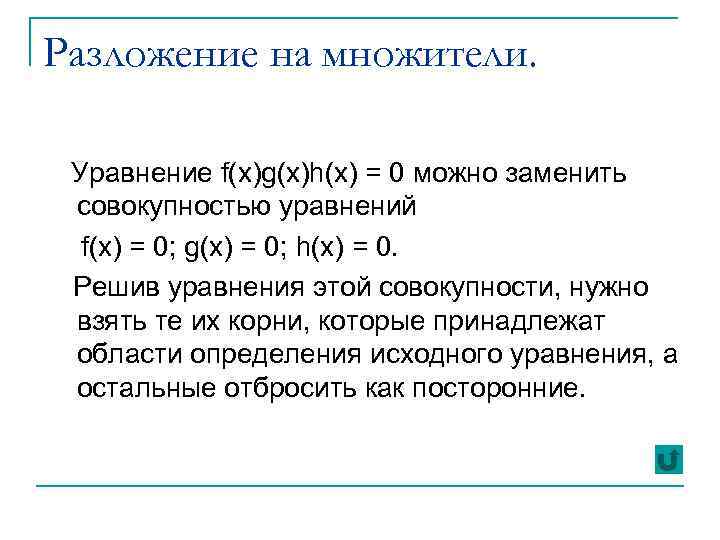Factorization. The equation f (x) g (x) h (x) = 0 can be replaced by a set of equations f (x) = 0; g (x) = 0; h (x) = 0. Having solved the equations of this set, you need to take those roots that belong to the domain of the original equation, and discard the rest as extraneous.

Solve the equation x³ - 7 x + 6 = 0 Representing the term 7 x as x + 6 x, we get sequentially: x³ - x - 6 x + 6 = 0 x (x² - 1) - 6 (x - 1) = 0 x (x - 1) (x + 1) - 6 (x - 1) = 0 (x - 1) (x² + x - 6) = 0 Now the problem is reduced to solving the set of equations x - 1 = 0; x² + x - 6 = 0. Answer: 1, 2, - 3.

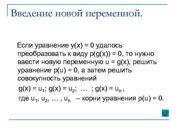Introducing a new variable. If the equation y (x) = 0 can be transformed to the form p (g (x)) = 0, then you need to introduce a new variable u = g (x), solve the equation p (u) = 0, and then solve the set of equations g ( x) = u 1; g (x) = u 2; ...; g (x) = un, where u 1, u 2,…, un are the roots of the equation p (u) = 0.

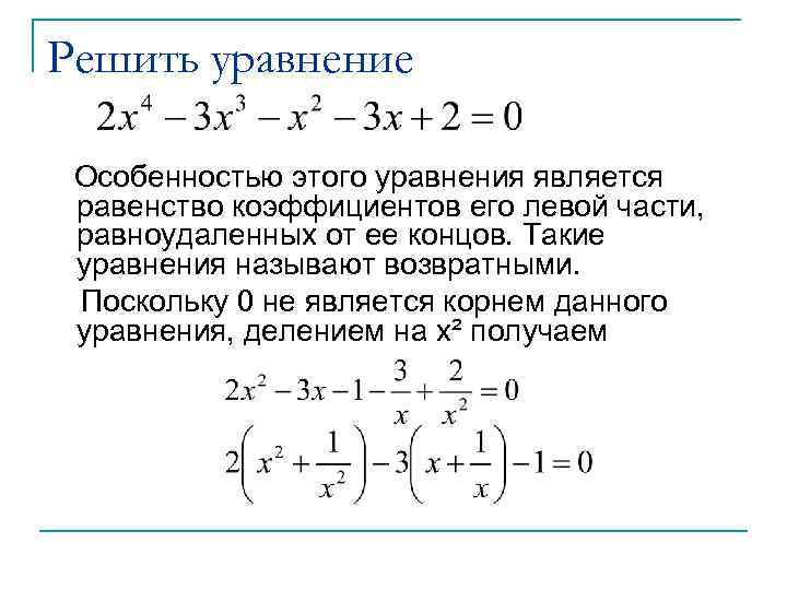Solve the equation A feature of this equation is the equality of the coefficients of its left side, equidistant from its ends. Such equations are called recurrent. Since 0 is not a root of this equation, dividing by x² we get

Let's introduce a new variable Then We get a quadratic equation So the root y 1 = - 1 can be ignored. We get the Answer: 2, 0, 5.

Solve the equation 6 (x² - 4) ² + 5 (x² - 4) (x² - 7 x +12) + (x² - 7 x + 12) ² = 0 This equation can be solved as homogeneous. Divide both sides of the equation by (x² - 7 x +12) ² (clearly, the values of x such that x² - 7 x + 12 = 0 are not solutions). Now let us denote We have Hence the Answer:

Functionally - graphical method. If one of the functions y = f (x), y = g (x) increases, and the other decreases, then the equation f (x) = g (x) either has no roots or has one root.

Solve the Equation It is fairly obvious that x = 2 is the root of the equation. Let us prove that this is the only root. We transform the equation to the form Note that the function increases and the function decreases. Hence, the equation has only one root. Answer: 2.

Selection of roots n n n Theorem 1: If an integer m is a root of a polynomial with integer coefficients, then the free term of the polynomial is divisible by m. Theorem 2: The reduced polynomial with integer coefficients has no fractional roots. Theorem 3: - an equation with integers Let the coefficients. If the number and fraction where p and q are integers is irreducible, is the root of the equation, then p is the divisor of the free term an, and q is the divisor of the coefficient at the leading term a 0.

Bezout's theorem. The remainder when dividing any polynomial by a binomial (x - a) is equal to the value of the divisible polynomial at x = a. Consequences of Bezout's theorem n n n n The difference of the same powers of two numbers is divisible without remainder by the difference of the same numbers; The difference of the same even powers of two numbers is divided without a remainder both by the difference of these numbers and by their sum; The difference of the same odd powers of two numbers is not divisible by the sum of these numbers; The sum of the same powers of two non-numbers is divided by the difference of these numbers; The sum of the same odd powers of two numbers is divided without a remainder by the sum of these numbers; The sum of the same even powers of two numbers is not divisible either by the difference of these numbers or by their sum; A polynomial is divisible entirely by a binomial (x - a) if and only if the number a is a root of the given polynomial; The number of distinct roots of a nonzero polynomial is at most its degree.

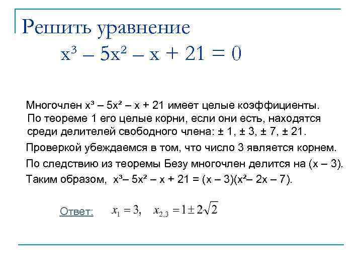Solve the equation x³ - 5 x² - x + 21 = 0 The polynomial x³ - 5 x² - x + 21 has integer coefficients. By Theorem 1, its integer roots, if any, are among the divisors of the free term: ± 1, ± 3, ± 7, ± 21. By checking, we make sure that the number 3 is a root. By the corollary to Bezout's theorem, the polynomial is divisible by (x - 3). So x³– 5 x² - x + 21 = (x - 3) (x²– 2 x - 7). Answer:

Solve the equation 2 x³ - 5 x² - x + 1 = 0 According to Theorem 1, the integer roots of the equation can only be numbers ± 1. The check shows that these numbers are not roots. Since the equation is not reduced, it can have fractional rational roots. Let's find them. To do this, multiply both sides of the equation by 4: 8 x³ - 20 x² - 4 x + 4 = 0 Making the substitution 2 x = t, we get t³ - 5 t² - 2 t + 4 = 0. By Theorem 2, all rational roots of this reduced equation must be whole. They can be found among the divisors of the free term: ± 1, ± 2, ± 4. In this case, t = - 1. Therefore, by the corollary of the Bezout theorem, the polynomial 2 x³ - 5 x² - x + 1 is divisible by (x + 0, 5 ): 2 x³ - 5 x² - x + 1 = (x + 0, 5) (2 x² - 6 x + 2) Solving the quadratic equation 2 x² - 6 x + 2 = 0, we find the remaining roots: Answer:

Solve the equation 6 x³ + x² - 11 x - 6 = 0 According to Theorem 3, the rational roots of this equation should be sought among the numbers Substituting them one by one into the equation, we find that satisfy the equation. They exhaust all the roots of the equation. Answer:

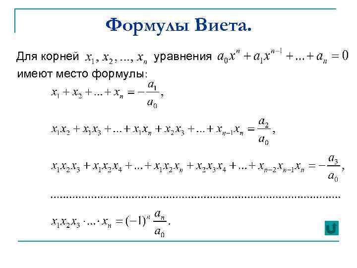
Find the sum of the squares of the roots of the equation x³ + 3 x² - 7 x +1 = 0 By Vieta's theorem Note that whence

Indicate which method can be used to solve each of these equations. Solve equations # 1, 4, 15, 17.

Answers and directions: 1. Introduction of a new variable. 2. Functional - graphic method. 3. Replacing the equation h (f (x)) = h (g (x)) by the equation f (x) = g (x). 4. Factorization. 5. Selection of roots. 6 Functional - graphical method. 7. Application of Vieta formulas. 8. Selection of roots. 9. Replacing the equation h (f (x)) = h (g (x)) by the equation f (x) = g (x). 10. Introduction of a new variable. 11. Factorization. 12. Introduction of a new variable. 13. Selection of roots. 14. Application of Vieta formulas. 15. Functional - graphic method. 16. Factorization. 17. Introducing a new variable. 18. Factorization.

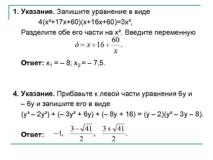1. Indication. Write the equation as 4 (x² + 17 x + 60) (x + 16 x + 60) = 3 x², Divide both sides by x². Enter the variable Answer: x 1 = - 8; x 2 = - 7, 5. 4. Note. Add 6 y and - 6 y to the left side of the equation and write it as (y³ - 2 y²) + (- 3 y² + 6 y) + (- 8 y + 16) = (y - 2) (y² - 3 y - eight). Answer:

14. Indication. By Vieta's theorem Since are integers, the roots of the equation can only be numbers - 1, - 2, - 3. Answer: 15. Answer: - 1. 17. Indication. Divide both sides of the equation by x² and write it as Enter variable Answer: 1; 15; 2; 3.

Bibliography. n n n Kolmogorov A. N. "Algebra and the beginning of analysis, 10 - 11" (Moscow: Education, 2003). Bashmakov M. I. "Algebra and the beginning of analysis, 10 - 11" (Moscow: Education, 1993). Mordkovich A. G. "Algebra and the beginning of analysis, 10 - 11" (M.: Mnemozina, 2003). Alimov Sh. A., Kolyagin Yu. M. et al. "Algebra and the beginning of analysis, 10 - 11" (Moscow: Education, 2000). Galitskiy ML, Gol'dman AM, Zvavich LI "Collection of problems in algebra, 8 - 9" (Moscow: Education, 1997). Karp A. P. "Collection of problems in algebra and the principles of analysis, 10 - 11" (Moscow: Education, 1999). Sharygin I. F. "Optional course in mathematics, problem solving, 10" (Moscow: Education. 1989). Skopets ZA "Additional chapters on the course of mathematics, 10" (Moscow: Education, 1974). Litinsky G. I. "Lessons of Mathematics" (M.: Aslan, 1994). Muravin G. K. "Equations, inequalities and their systems" (Mathematics, supplement to the newspaper "September 1", No. 2, 3, 2003). Kolyagin Yu. M. “Polynomials and equations higher degrees"(Mathematics, supplement to the newspaper" September 1 ", No. 3, 2005).

The text of the work is placed without images and formulas.
Full version work is available in the tab "Files of work" in PDF format

Introduction

Solving algebraic equations of higher degrees with one unknown is one of the most difficult and ancient mathematical problems... The most outstanding mathematicians of antiquity were engaged in these problems.

Solving equations of the n-th degree is an important task for modern mathematics as well. Interest in them is quite large, since these equations are closely related to the search for the roots of equations that are not considered in the school curriculum in mathematics.

Problem: the lack of skills in solving equations of higher degrees in various ways among students prevents them from successfully preparing for the final certification in mathematics and mathematical olympiads, teaching in a specialized mathematical class.

The listed facts determined relevance of our work "Solving equations of higher degrees."

Possession of the simplest ways to solve equations of the n-th degree reduces the time to complete the task, on which the result of the work and the quality of the learning process depend.

Purpose of work: the study known methods solving equations of higher degrees and identifying the most accessible ones for practical application.

Based on this goal, the work identified the following tasks:

Study literature and Internet resources on this topic;

Get acquainted with the historical facts related to this topic;

Describe the different ways to solve higher-degree equations

compare the degree of complexity of each of them;

To acquaint classmates with methods of solving equations of higher degrees;

Create a set of equations for the practical application of each of the considered methods.

Object of study- equations of higher degrees with one variable.

Subject of study- ways to solve equations of higher degrees.

Hypothesis: there is no general method and unified algorithm that allows finding solutions to equations of the n-th degree in a finite number of steps.

Research methods:

- bibliographic method (analysis of literature on the research topic);

- classification method;

- method of qualitative analysis.

Theoretical significance research consists in the systematization of methods for solving equations of higher degrees and the description of their algorithms.

Practical significance- the presented material on this topic and the development of a textbook for students on this topic.

1 HIGHER DEGREES EQUATIONS

1.1 The concept of an equation of the n-th degree

Definition 1. An equation of the nth degree is an equation of the form

a 0 xⁿ + a 1 x n -1 + a 2 xⁿ - ² + ... + a n -1 x + a n = 0, where the coefficients a 0, a 1, a 2…, a n -1, a n- any real numbers, and , a 0 ≠ 0 .

Polynomial a 0 xⁿ + a 1 x n -1 + a 2 xⁿ - ² + ... + a n -1 x + a n is called a polynomial of degree n. The coefficients are distinguished by their names: a 0 - senior coefficient; a n is a free member.

Definition 2. Solutions or roots for a given equation are all values of the variable NS, which turn this equation into a true numerical equality or, in which the polynomial a 0 xⁿ + a 1 x n -1 + a 2 xⁿ - ² + ... + a n -1 x + a n vanishes. This value of the variable NS is also called the root of the polynomial. To solve an equation means to find all its roots or to establish that they do not exist.

If a 0 = 1, then such an equation is called the reduced whole rational equation n th degree.

For equations of the third and fourth degrees, Cardano's and Ferrari's formulas exist, expressing the roots of these equations in terms of radicals. It turned out that in practice they are rarely used. Thus, if n ≥ 3, and the coefficients of the polynomial are arbitrary real numbers, then finding the roots of the equation is not an easy task. Nevertheless, in many special cases, this problem is solved to the end. Let's dwell on some of them.

1.2 Historical facts solutions of equations of higher degrees

Already in ancient times, people realized how important it is to learn how to solve algebraic equations. About 4,000 years ago, Babylonian scholars possessed the solution quadratic equation and solved a system of two equations, one of which is of the second degree. With the help of equations of higher degrees, various problems of land surveying, architecture and military affairs were solved, many and various questions of practice and natural science were reduced to them, since the exact language of mathematics allows you to simply express facts and relationships that, being presented in ordinary language, may seem confusing and complicated ...

Universal formula for finding roots algebraic equation nth degree no. Many, of course, came up with the tempting idea to find for any power n formulas that would express the roots of the equation in terms of its coefficients, that is, would solve the equation in radicals.

Only in the 16th century did Italian mathematicians succeed in moving forward - to find formulas for n = 3 and n = 4. At the same time, the question of general decision equations of the 3rd degree were studied by Scipio, Dahl, Ferro and his students Fiori and Tartaglia.

In 1545, the book of the Italian mathematician D. Cardano "The Great Art, or the Rules of Algebra" was published, where, along with other questions of algebra, general methods of solving cubic equations were considered, as well as the method for solving equations of the 4th degree, discovered by his student L. Ferrari.

F. Viet gave a complete exposition of questions related to the solution of equations of the third and fourth degrees.

In the 20s of the 19th century, the Norwegian mathematician N. Abel proved that the roots of equations of the fifth degree cannot be expressed in terms of radicals.

The study revealed that modern science there are many ways to solve equations of the n-th degree.

The result of the search for methods for solving equations of higher degrees that cannot be solved by the methods considered in school curriculum, methods based on the application of Vieta's theorem (for equations of degree n> 2), Bezout's theorems, Horner's schemes, as well as the Cardano and Ferrari formula for solving cubic equations and equations of the fourth degree.

The paper presents methods for solving equations and their types, which became a discovery for us. These include - the method of indefinite coefficients, the selection of the full degree, symmetric equations.

2. SOLUTION OF INTEGER EQUATIONS OF HIGHER DEGREES WITH INTEGER COEFFICIENTS

2.1 Solving 3rd degree equations. Formula D. Cardano

Consider equations of the form x 3 + px + q = 0. We transform the general equation to the form: x 3 + px 2 + qx + r = 0. Let's write the formula for the sum cube; We add it to the original equality and replace it with y... We get the equation: y 3 + (q -) (y -) + (r - = 0. After transformations, we have: y 2 + py + q = 0. Now, again, write the formula for the sum cube:

(a + b) 3 = a 3 + 3a 2 b + 3ab 2 + b 3 = a 3 + b 3 + 3ab (a + b), replace ( a + b)on x, we get the equation x 3 - 3abx - (a 3 + b 3) = 0. Now you can see that the original equation is equivalent to the system: and Solving the system, we get:

We have obtained a formula for solving the reduced equation of the 3rd degree. She bears the name of the Italian mathematician Cardano.

Let's look at an example. Solve the equation:.

We have R= 15 and q= 124, then using the Cardano formula we calculate the root of the equation

Output: this formula good, but not good for solving all cubic equations. However, it is cumbersome. Therefore, in practice, it is rarely used.

But the one who masters this formula can use it when solving third-degree equations on the exam.

2.2 Vieta's theorem

From the course of mathematics, we know this theorem for a quadratic equation, but few people know that it is also used to solve equations of higher degrees.

Consider the equation:

factor the left side of the equation, divide by ≠ 0.

We transform the right side of the equation to the form

; from this it follows that the following equalities can be written into the system:

The formulas derived by Viet for quadratic equations and demonstrated by us for equations of the third degree are also true for polynomials of higher degrees.

Let's solve the cubic equation:

Output: this way universal and easy enough for students to understand, since Vieta's theorem is familiar to them from the school curriculum for n = 2. At the same time, in order to find the roots of equations using this theorem, one must have good computational skills.

2.3 Bezout's theorem

This theorem is named after the French mathematician of the 18th century J. Bezout.

Theorem. If the equation a 0 xⁿ + a 1 x n -1 + a 2 xⁿ - ² + ... + a n -1 x + a n = 0, in which all coefficients are integers, and the free term is nonzero, has an integer root, then this root is a divisor of the free term.

Considering that on the left side of the equation polynomial nth degree, then the theorem has a different interpretation.

Theorem. When dividing a polynomial nth degree relatively x binomial x - a the remainder is equal to the value of the dividend at x = a... (letter a can denote any real or imaginary number, i.e. any complex number).

Proof: let be f (x) denotes an arbitrary n-th degree polynomial with respect to the variable x, and let, when dividing by the binomial ( x-a) happened in private q (x), and in the remainder R... It's obvious that q (x) there will be some polynomial (n - 1) th degree with respect to x and the remainder R will be a constant value, i.e. independent of x.

If the remainder R was a polynomial of the first degree with respect to x, then this would mean that the division is not satisfied. So, R from x does not depend. By the definition of division, we obtain the identity: f (x) = (x-a) q (x) + R.

Equality is valid for any value of x, which means that it is also valid for x = a, we get: f (a) = (a-a) q (a) + R... Symbol f (a) denotes the value of the polynomial f (x) at x = a, q (a) denotes the value q (x) at x = a. Remainder R remained the same as it was before, since R from x does not depend. Work ( x-a) q (a) = 0, since the factor ( x-a) = 0, and the factor q (a) there is a certain number. Therefore, from the equality we get: f (a) = R, h.t.d.

Example 1. Find the remainder of the division of a polynomial x 3 - 3x 2 + 6x- 5 for binomial

x- 2. By Bezout's theorem : R = f(2) = 23-322 + 62 -5 = 3. Answer: R = 3.

Note that Bezout's theorem is important not so much in itself as in its consequences. (Annex 1)

Let us dwell on some methods of applying Bezout's theorem to solving practical problems. It should be noted that when solving equations using Bezout's theorem, it is necessary:

Find all integer divisors of the free term;

Find at least one root of the equation from these divisors;

Divide the left side of the equation by (Ha);

Write down the product of the divisor and the quotient on the left side of the equation;

Solve the resulting equation.

Consider, for example, solving the equation x 3 + 4NS 2 + x - 6 = 0 .

Solution: find the divisors of the free term ± 1 ; ± 2; ± 3; ± 6. Let us calculate the values at x = 1, 1 3 + 41 2 + 1- 6 = 0. Divide the left side of the equation by ( NS- 1). We will perform the division "with a corner", we get:

Conclusion: Bezout's theorem, one of the ways that we consider in our work, is studied in the program of optional classes. It is difficult to understand, because in order to own it, you need to know all the consequences from it, but at the same time Bezout's theorem is one of the main assistants of students on the exam.

2.4 Horner's scheme

To divide a polynomial by a binomial x-α you can use a special simple trick invented by English mathematicians of the 17th century, later called Horner's scheme. In addition to finding the roots of equations, according to Horner's scheme, it is easier to calculate their values. For this, it is necessary to substitute the value of the variable into the polynomial Pn (x) = a 0 xn + a 1 x n-1 + a 2 xⁿ - ² +… ++ a n -1 x + a n. (1)

Consider the division of the polynomial (1) by the binomial x-α.

Let us express the coefficients of the incomplete quotient b 0 xⁿ - ¹+ b 1 xⁿ - ²+ b 2 xⁿ - ³+…+ bn -1 and the remainder r in terms of the coefficients of the polynomial Pn ( x) and the number α. b 0 = a 0 , b 1 = α b 0 + a 1 , b 2 = α b 1 + a 2 …, bn -1 =

= α bn -2 + a n -1 = α bn -1 + a n .

Calculations according to Horner's scheme are presented in the form of the following table:

	a 0	a 1	a 2 ,
	b 0 = a 0	b 1 = α b 0 + a 1	b 2 = α b 1 + a 2		r = α b n-1 + a n

Insofar as r = Pn (α), then α is the root of the equation. In order to check whether α is a multiple root, Horner's scheme can be applied to the quotient b 0 x + b 1 x + ... + bn -1 according to the table. If in the column below bn -1 it will turn out to be 0 again, which means that α is a multiple root.

Consider an example: Solve the equation NS 3 + 4NS 2 + x - 6 = 0.

Apply the factorization of the polynomial on the left side of the equation, Horner's scheme to the left side of the equation.

Solution: find the divisors of the free term ± 1; ± 2; ± 3; ± 6.


				6 ∙ 1 + (-6) = 0

The quotients are numbers 1, 5, 6, and the remainder is r = 0.

Means, NS 3 + 4NS 2 + NS - 6 = (NS - 1) (NS 2 + 5NS + 6) = 0.

Hence: NS- 1 = 0 or NS 2 + 5NS + 6 = 0.

NS = 1, NS 1 = -2; NS 2 = -3. Answer: 1,- 2, - 3.

Conclusion: thus, on one equation, we showed the application of two different ways factoring polynomials. In our opinion, Horner's scheme is the most practical and economical.

2.5 Solving equations of the 4th degree. Ferrari method

Cardano's student Ludovic Ferrari discovered a way to solve the 4th degree equation. The Ferrari method consists of two steps.

Stage I: equations of the form are represented in the form of a product of two square trinomials, this follows from the fact that the equation is of the 3rd degree and at least one solution.

Stage II: the obtained equations are solved using factorization, however, in order to find the required factorization, it is necessary to solve cubic equations.

The idea is to represent the equations in the form A 2 = B 2, where A = x 2 + s,

B-linear function of x... Then it remains to solve the equations A = ± B.

For clarity, consider the equation: Let us isolate the 4th degree, we get: For any d the expression will be a perfect square. Add to both sides of the equation we get

On the left side there is a full square, you can pick up d so that the right-hand side (2) also becomes a complete square. Let's imagine that we have achieved this. Then our equation looks like this:

Finding the root afterwards will not be difficult. To choose the right one d it is necessary that the discriminant of the right-hand side (3) vanish, i.e.

So to find d, it is necessary to solve this equation of the 3rd degree. Such an auxiliary equation is called resolution.

We can easily find the whole root of the resolvent: d = 1

Substituting the equation into (1), we obtain

Conclusion: Ferrari's method is universal, but complicated and cumbersome. At the same time, if the solution algorithm is clear, then 4th degree equations can be solved by this method.

2.6 Method of undefined coefficients

The success of solving the equation of the 4th degree by the Ferrari method depends on whether we solve the resolvent - the equation of the 3rd degree, which, as we know, is not always possible.

The essence of the method of undefined coefficients is that the type of factors into which a given polynomial is decomposed is guessed, and the coefficients of these factors (also polynomials) are determined by multiplying the factors and equating the coefficients at the same degrees of the variable.

Example: Solve the equation:

Suppose that the left-hand side of our equation can be decomposed into two square trinomials with integer coefficients such that the identity

Obviously, the coefficients in front of the uni should be equal to 1, and the free terms should be equal to one + 1, the other has 1.

The coefficients in front of NS... Let us denote them by a and and to determine them, we multiply both trinomials on the right side of the equation.

As a result, we get:

Equating the coefficients at the same degrees NS in the left and right sides equality (1), we obtain a system for finding and

Having solved this system, we will have

So, our equation is equivalent to the equation

Having solved it, we get the following roots:.

The method of indefinite coefficients is based on the following statements: any polynomial of the fourth degree in the equation can be decomposed into the product of two polynomials of the second degree; two polynomials are identically equal if and only if their coefficients are equal at the same degrees NS.

2.7 Symmetric Equations

Definition. An equation of the form is called symmetric if the first coefficients on the left in the equation are equal to the first coefficients on the right.

We see that the first coefficients on the left are equal to the first coefficients on the right.

If such an equation has an odd degree, then it has the root NS= - 1. Next, we can lower the degree of the equation by dividing it by ( x + 1). It turns out that when the symmetric equation is divided by ( x + 1) a symmetric equation of even degree is obtained. The proof of the symmetry of the coefficients is presented below. (Appendix 6) Our task is to learn how to solve symmetric equations of even degree.

For example: (1)

We solve equation (1), divide by NS 2 (medium) = 0.

Let us group the terms with symmetric

) + 3(x+. We denote at= x+, we will square both sides, hence = at 2 So, 2 ( at 2 or 2 at 2 + 3 solving the equation, we get at = , at= 3. Next, let's go back to replacing x+ = and x+ = 3. We get the equations and The first has no solution, and the second has two roots. Answer:.

Output: given view equations are not often encountered, but if you come across it, then it can be solved easily and simply without resorting to cumbersome calculations.

2.8 Isolation of the full degree

Consider the equation.

The left side is the cube of the sum (x + 1), i.e.

We extract the root of the third degree from both parts:, then we get

Where is the only root.

RESULTS OF THE STUDY

Based on the results of the work, we came to the following conclusions:

Thanks to the studied theory, we got acquainted with different methods solutions of entire equations of higher degrees;

D. Cardano's formula is difficult to apply and gives a high probability of making errors in the calculation;

- L. Ferrari's method makes it possible to reduce the solution of an equation of the fourth degree to a cubic one;

- Bezout's theorem can be applied both for cubic equations and for equations of the fourth degree; it is more understandable and visual when applied to the solution of equations;

Horner's scheme helps to significantly reduce and simplify calculations in solving equations. In addition to finding the roots, according to Horner's scheme, it is easier to calculate the values of the polynomials on the left side of the equation;

Of particular interest was the solution of equations by the method of undefined coefficients, the solution of symmetric equations.

During research work it was found that students get acquainted with the simplest methods of solving equations of the highest degree in the elective classes in mathematics, starting from the 9th or 10th grade, as well as in special courses outside mathematics schools... This fact was established as a result of a survey of mathematics teachers at MBOU "Secondary School No. 9" and students showing an increased interest in the subject of "mathematics".

The most popular methods for solving equations of higher degrees, which are found in solving Olympiad, competitive problems and as a result of student preparation for exams, are methods based on the application of Bezout's theorem, Horner's scheme and the introduction of a new variable.

Demonstration of the results of research work, i.e. ways to solve equations that are not studied in the school curriculum in mathematics, interested classmates.

Conclusion

Having studied educational and scientific literature, Internet resources in youth educational forums

In general, an equation with a degree higher than 4 cannot be solved in radicals. But sometimes we can still find the roots of the polynomial on the left in the equation of the highest degree, if we represent it as a product of polynomials in degree at most 4. The solution to such equations is based on factoring a polynomial into factors, so we advise you to repeat this topic before studying this article.

Most often one has to deal with equations of higher degrees with integer coefficients. In these cases, we can try to find the rational roots, and then factor the polynomial in order to then transform it into an equation of a lower degree, which will be easy to solve. Within the framework of this material, we will consider just such examples.

Yandex.RTB R-A-339285-1

Equations of the highest degree with integer coefficients

All equations of the form a n x n + a n - 1 x n - 1 +. ... ... + a 1 x + a 0 = 0, we can reduce to an equation of the same degree by multiplying both sides by a n n - 1 and changing a variable of the form y = a n x:

a n x n + a n - 1 x n - 1 +. ... ... + a 1 x + a 0 = 0 ann xn + an - 1 ann - 1 xn - 1 +… + a 1 (an) n - 1 x + a 0 (an) n - 1 = 0 y = anx ⇒ yn + bn - 1 yn - 1 +… + b 1 y + b 0 = 0

The resulting coefficients will also be whole. Thus, we will need to solve the reduced equation of the nth degree with integer coefficients, which has the form x n + a n x n - 1 +… + a 1 x + a 0 = 0.

We calculate the whole roots of the equation. If the equation has integer roots, you need to look for them among the divisors of the free term a 0. Let us write them down and substitute them into the original equality in turn, checking the result. Once we have obtained an identity and found one of the roots of the equation, we can write it in the form x - x 1 · P n - 1 (x) = 0. Here x 1 is the root of the equation, and P n - 1 (x) is the quotient of dividing x n + a n x n - 1 +… + a 1 x + a 0 by x - x 1.

Substitute the rest of the divisors written out in P n - 1 (x) = 0, starting with x 1, since the roots can be repeated. After obtaining the identity, the root x 2 is considered found, and the equation can be written as (x - x 1) (x - x 2) P n - 2 (x) = 0. Here P n - 2 (x) will be the quotient of dividing P n - 1 (x) by x - x 2.

We continue to iterate over the divisors. Find all whole roots and denote their number as m. After that, the original equation can be represented as x - x 1 x - x 2 · ... · x - x m · P n - m (x) = 0. Here P n - m (x) is a polynomial of degree n - m. It is convenient to use Horner's scheme for counting.

If our original equation has integer coefficients, we cannot end up with fractional roots.

As a result, we got the equation P n - m (x) = 0, the roots of which can be found by any in a convenient way... They can be irrational or complex.

Let's show on specific example how such a solution scheme is applied.

Example 1

Condition: find the solution to the equation x 4 + x 3 + 2 x 2 - x - 3 = 0.

Solution

Let's start by finding whole roots.

We have a free term equal to minus three. It has divisors of 1, - 1, 3, and - 3. Let's substitute them in the original equation and see which of them will result in identities.

With x equal to one, we get 1 4 + 1 3 + 2 · 1 2 - 1 - 3 = 0, which means that one will be the root of this equation.

Now we perform division of the polynomial x 4 + x 3 + 2 x 2 - x - 3 by (x - 1) in a column:

Hence, x 4 + x 3 + 2 x 2 - x - 3 = x - 1 x 3 + 2 x 2 + 4 x + 3.

1 3 + 2 1 2 + 4 1 + 3 = 10 ≠ 0 (- 1) 3 + 2 (- 1) 2 + 4 - 1 + 3 = 0

We have obtained an identity, which means that we have found another root of the equation, equal to - 1.

Divide the polynomial x 3 + 2 x 2 + 4 x + 3 by (x + 1) in a column:

We get that

x 4 + x 3 + 2 x 2 - x - 3 = (x - 1) (x 3 + 2 x 2 + 4 x + 3) = = (x - 1) (x + 1) (x 2 + x + 3)

Substitute the next divisor into the equality x 2 + x + 3 = 0, starting with - 1:

1 2 + (- 1) + 3 = 3 ≠ 0 3 2 + 3 + 3 = 15 ≠ 0 (- 3) 2 + (- 3) + 3 = 9 ≠ 0

The resulting equalities will be incorrect, which means that the equation no longer has integral roots.

The remaining roots will be the roots of the expression x 2 + x + 3.

D = 1 2 - 4 1 3 = - 11< 0

It follows from this that this square trinomial has no real roots, but has complex conjugate ones: x = - 1 2 ± i 11 2.

Let us clarify that instead of long division, Horner's scheme can be used. This is done like this: after we have determined the first root of the equation, we fill in the table.

In the table of coefficients, we can immediately see the coefficients of the quotient of the division of polynomials, which means that x 4 + x 3 + 2 x 2 - x - 3 = x - 1 x 3 + 2 x 2 + 4 x + 3.

After finding the next root equal to - 1, we get the following:

Answer: x = - 1, x = 1, x = - 1 2 ± i 11 2.

Example 2

Condition: Solve the equation x 4 - x 3 - 5 x 2 + 12 = 0.

Solution

The free term has divisors 1, - 1, 2, - 2, 3, - 3, 4, - 4, 6, - 6, 12, - 12.

We check them in order:

1 4 - 1 3 - 5 1 2 + 12 = 7 ≠ 0 (- 1) 4 - (- 1) 3 - 5 (- 1) 2 + 12 = 9 ≠ 0 2 4 2 3 - 5 2 2 + 12 = 0

Hence, x = 2 will be the root of the equation. Divide x 4 - x 3 - 5 x 2 + 12 by x - 2 using Horner's scheme:

As a result, we get x - 2 (x 3 + x 2 - 3 x - 6) = 0.

2 3 + 2 2 - 3 2 - 6 = 0

Hence, 2 will again be a root. Divide x 3 + x 2 - 3 x - 6 = 0 by x - 2:

As a result, we get (x - 2) 2 (x 2 + 3 x + 3) = 0.

It makes no sense to check the remaining divisors, since the equality x 2 + 3 x + 3 = 0 is faster and more convenient to solve using the discriminant.

Let's solve the quadratic equation:

x 2 + 3 x + 3 = 0 D = 3 2 - 4 1 3 = - 3< 0

We get a complex conjugate pair of roots: x = - 3 2 ± i 3 2.

Answer: x = - 3 2 ± i 3 2.

Example 3

Condition: find the real roots for the equation x 4 + 1 2 x 3 - 5 2 x - 3 = 0.

Solution

x 4 + 1 2 x 3 - 5 2 x - 3 = 0 2 x 4 + x 3 - 5 x - 6 = 0

We carry out multiplication 2 3 of both sides of the equation:

2 x 4 + x 3 - 5 x - 6 = 0 2 4 x 4 + 2 3 x 3 - 20 2 x - 48 = 0

Replace the variables y = 2 x:

2 4 x 4 + 2 3 x 3 - 20 2 x - 48 = 0 y 4 + y 3 - 20 y - 48 = 0

As a result, we got a standard 4th degree equation that can be solved according to the standard scheme. Let's check the divisors, divide and get in the end that it has 2 real roots y = - 2, y = 3 and two complex roots. We will not present the complete solution here. Due to the replacement, the real roots of this equation will be x = y 2 = - 2 2 = - 1 and x = y 2 = 3 2.

Answer: x 1 = - 1, x 2 = 3 2

If you notice an error in the text, please select it and press Ctrl + Enter

Marina A. Trifanova
teacher of mathematics, MOU "Gymnasium No. 48 (multidisciplinary)", Talnakh

The triune goal of the lesson:

Educational:
systematization and generalization of knowledge on the solution of equations of higher degrees.
Developing:
promote the development logical thinking, the ability to work independently, the skills of mutual control and self-control, the ability to speak and listen.
Educational:
developing a habit of constant employment, fostering responsiveness, hard work, accuracy.

Lesson type:

a lesson in the complex application of knowledge, skills and abilities.

Lesson form:

airing, physical training, various forms of work.

Equipment:

supporting notes, cards with assignments, lesson monitoring matrix.

DURING THE CLASSES

I. Organizational moment

Communicating the lesson goal to students.
Homework check (Appendix 1). Work with reference notes (Appendix 2).

Equations and answers for each of them are written on the board. Students check the answers and give brief analysis solutions to each equation or answer the teacher's questions (frontal survey). Self-control - students give themselves grades and hand over exercise books to the teacher to correct or approve grades. The grade school is written on the chalkboard:

“5+” - 6 equations;
“5” - 5 equations;
“4” - 4 equations;
“3” - 3 equations.

Teacher's homework questions:

1 equation

What change of variables is made in the equation?
What equation is obtained after changing variables?

2 equation

What polynomial did both sides of the equation divide into?
What change of variables was obtained?

3 equation

What polynomials do you need to multiply to simplify the solution of this equation?

4 equation

Name the function f (x).
How were the rest of the roots found?

Equation 5

How many gaps were obtained to solve the equation?

6 equation

In what ways could this equation be solved?
Which solution is more rational?

II. Group work is the main part of the lesson.

The class is divided into 4 groups. Each group is given a card with theoretical and practical (Appendix 3) questions: "Deconstruct the proposed method for solving the equation and explain it using this example."

Group work 15 minutes.
Examples are written on the board (the board is divided into 4 parts).
The group report takes 2 - 3 minutes.
The teacher corrects the reports of the groups and helps in case of difficulty.

The group work continues on cards 5 - 8. Each equation is given 5 minutes for group discussion. Then the board has a report on this equation- a brief analysis of the solution. The equation may not be completely solved - it is being finalized at home, but the sequence of its solution in the classroom is discussed all over.

III. Independent work. Appendix 4.

Each student receives an individual assignment.
Time work takes 20 minutes.
5 minutes before the end of the lesson, the teacher gives open-ended answers for each equation.
Students change notebooks in a circle and check the answers from a friend. Give marks.
Notebooks are handed over to the teacher for checking and correcting grades.

IV. Lesson summary.

Homework.

Checkout the solution to unfinished equations. Prepare for a control slice.

Grading.

Basic goals:

To consolidate the concept of a whole rational equation of the th degree.
Formulate the main methods for solving equations of higher degrees (n > 3).
To teach the basic methods of solving equations of higher degrees.
To teach by the type of equation to determine the most effective method his decisions.

Forms, methods and pedagogical techniques that are used by the teacher in the lesson:

Lecture-seminar training system (lectures - explanation of new material, seminars - problem solving).
Information and communication technologies (frontal survey, oral work with the class).
Differentiated learning, group and individual forms.
The use of a research method in teaching, aimed at developing the mathematical apparatus and thinking abilities of each specific student.
Printed material - individual short synopsis lesson (basic concepts, formulas, statements, lecture material is compressed in the form of diagrams or tables).

Lesson plan:

Organizing time.
Stage goal: to include students in learning activities, determine the meaningful framework of the lesson.
Updating students' knowledge.
The purpose of the stage: to update the knowledge of students on previously studied related topics
The study new topic(lecture). The purpose of the stage: to formulate the main methods for solving equations of higher degrees (n > 3)
Summarizing.
The purpose of the stage: once again highlight the key points in the material studied in the lesson.
Homework.
Stage goal: to formulate homework for students.

Lesson summary

1. Organizational moment.

Formulation of the topic of the lesson: “Equations of the highest degrees. Methods for their solution ”.

2. Actualization of students' knowledge.

Theoretical survey - conversation. Repetition of some previously studied information from the theory. Students formulate basic definitions and formulate necessary theorems. Examples are given to demonstrate the level of knowledge gained earlier.

The concept of an equation in one variable.
The concept of the root of the equation, the solution of the equation.
Concept linear equation with one variable, the concept of a quadratic equation in one variable.
The concept of equivalence of equations, equation-consequence (concept of extraneous roots), transition not by consequence (the case of loss of roots).
The concept of a whole rational expression with one variable.
The concept of a whole rational equation n-th degree. The standard form of the whole rational equation. Reduced whole rational equation.
The transition to a set of equations is more low degrees by factoring the original equation.
Polynomial concept n-th degree from x... Bezout's theorem. Consequences from Bezout's theorem. Root theorems ( Z-roots and Q-roots) of an entire rational equation with integer coefficients (reduced and non-reduced, respectively).
Horner's scheme.

3. Studying a new topic.

We will consider the whole rational equation n-th degree of the standard form with one unknown variable x: P n (x)= 0, where P n (x) = a n x n + a n-1 x n-1 + a 1 x + a 0- polynomial n-th degree from x, a n ≠ 0. If a n = 1 then such an equation is called the reduced whole rational equation n-th degree. Consider such equations for different meanings n and list the main methods for solving them.

n= 1 - linear equation.

n= 2 - quadratic equation. Discriminant formula. Formula for calculating roots. Vieta's theorem. Selecting a complete square.

n= 3 - cubic equation.

Grouping method.

Example: x 3 - 4x 2 - x+ 4 = 0 (x - 4) (x 2– 1) = 0 x 1 = 4 , x 2 = 1,x 3 = -1.

Reverse cubic equation of the form ax 3 + bx 2 + bx + a= 0. Solve by combining terms with the same coefficients.

Example: x 3 – 5x 2 – 5x + 1 = 0 (x + 1)(x 2 – 6x + 1) = 0 x 1 = -1, x 2 = 3 + 2, x 3 = 3 – 2.

Selection of Z-roots based on the theorem. Horner's scheme. When applying this method, it is necessary to emphasize that the search in this case is finite, and we select the roots according to a certain algorithm in accordance with the theorem on Z-roots of the reduced whole rational equation with integer coefficients.

Example: x 3 – 9x 2 + 23x- 15 = 0. Equation given. Let us write down the divisors of the free term ( + 1; + 3; + 5; + 15). Let's apply Horner's scheme:

	x 3	x 2	x 1	x 0	output
	1	-9	23	-15
1	1	1 x 1 - 9 = -8	1 x (-8) + 23 = 15	1 x 15 - 15 = 0	1 - root
	x 2	x 1	x 0

We get ( x – 1)(x 2 – 8x + 15) = 0 x 1 = 1, x 2 = 3, x 3 = 5.

Equation with integer coefficients. Selection of Q-roots based on the theorem. Horner's scheme. When applying this method, it is necessary to emphasize that the enumeration in this case is finite and we select the roots according to a certain algorithm in accordance with the theorem on Q-roots of an irreducible entire rational equation with integer coefficients.

Example: 9 x 3 + 27x 2 – x- 3 = 0. The equation is not reduced. Let us write down the divisors of the free term ( + 1; + 3). Let us write down the divisors of the coefficient at the highest power of the unknown. ( + 1; + 3; + 9) Therefore, we will look for roots among the values ( + 1; + ; + ; + 3). Let's apply Horner's scheme:

	x 3	x 2	x 1	x 0	output
	9	27	-1	-3
1	9	1 x 9 + 27 = 36	1 x 36 - 1 = 35	1 x 35 - 3 = 32 ≠ 0	1 - not root
-1	9	-1 x 9 + 27 = 18	-1 x 18 - 1 = -19	-1 x (-19) - 3 = 16 ≠ 0	-1 - not root
	9	x 9 + 27 = 30	x 30 - 1 = 9	x 9 - 3 = 0	root
	x 2	x 1	x 0

We get ( x – )(9x 2 + 30x + 9) = 0 x 1 = , x 2 = - , x 3 = -3.

For the convenience of calculation when selecting Q -roots it can be convenient to make a change of variable, go to the reduced equation and select Z -roots.

If the free term is 1

.

If you can use a substitution of the form y = kx

.

Formula Cardano. Exists universal method solutions of cubic equations are Cardano's formula. This formula is associated with the names of Italian mathematicians Gerolamo Cardano (1501-1576), Nicolo Tartaglia (1500-1557), Scipiona del Ferro (1465-1526). This formula is outside the scope of our course.

n= 4 - equation of the fourth degree.

Grouping method.

Example: x 4 + 2x 3 + 5x 2 + 4x – 12 = 0 (x 4 + 2x 3) + (5x 2 + 10x) – (6x + 12) = 0 (x + 2)(x 3 + 5x - 6) = 0 (x + 2)(x– 1)(x 2 + x + 6) = 0 x 1 = -2, x 2 = 1.

Variable replacement method.

Biquadratic equation of the form ax 4 + bx 2 + s = 0 .

Example: x 4 + 5x 2 - 36 = 0. Substitution y = x 2. From here y 1 = 4, y 2 = -9. That's why x 1,2 = + 2 .

Reverse equation of the fourth degree of the form ax 4 + bx 3 + c x 2 + bx + a = 0.

We solve by combining terms with the same coefficients by replacing the form

ax 4 + bx 3 + cx 2 – bx + a = 0.

Generalized fourth-degree return equation of the form ax 4 + bx 3 + cx 2 + kbx + k 2 a = 0.

Replacement of the general view. Some standard replacements.

Example 3 . Replacing the general view(follows from the form of a specific equation).

n = 3.

Equation with integer coefficients. Fitting Q-roots n = 3.

General formula. There is a universal method for solving equations of the fourth degree. This formula is associated with the name of Ludovico Ferrari (1522-1565). This formula is outside the scope of our course.

n > 5 - equations of the fifth and higher degrees.

Equation with integer coefficients. Selection of Z-roots based on the theorem. Horner's scheme. The algorithm is similar to that considered above for n = 3.

Equation with integer coefficients. Fitting Q-roots based on the theorem. Horner's scheme. The algorithm is similar to that considered above for n = 3.

Symmetric equations. Any return equation of odd degree has a root x= -1 and after factoring it into factors, we obtain that one factor has the form ( x+ 1), and the second factor is the return equation of an even degree (its degree is one less than the degree of the original equation). Any return equation of even degree together with a root of the form x = φ also contains the root of the species. Using these statements, we solve the problem by lowering the degree of the equation under study.

Variable replacement method. Using uniformity.

There is no general formula for solving entire equations of the fifth degree (this was shown by the Italian mathematician Paolo Ruffini (1765-1822) and the Norwegian mathematician Niels Henrik Abel (1802-1829)) and higher degrees (this was shown by the French mathematician Evariste Galois (1811-1832) )).

Let us recall again that in practice it is possible to use combinations methods listed above. It is convenient to go over to a set of equations of lower degrees by factorization of the original equation.
Widely used in practice remained outside the scope of our today's discussion. graphic methods solving equations and approximate solution methods equations of higher degrees.

There are situations when the equation has no R-roots.

Using the monotonicity property of functions

4. Summing up.

Summary: Now we have mastered the basic methods of solving various equations of higher degrees (for n > 3). Our task is to learn how to effectively use the algorithms listed above. Depending on the type of equation, we will have to learn to determine which solution method in this case is the most effective, as well as correctly apply the chosen method.

5. Homework.

: p. 7, p. 164-174, No. 33-36, 39-44, 46.47.

: №№ 9.1–9.4, 9.6–9.8, 9.12, 9.14–9.16, 9.24–9.27.

Possible topics of reports or abstracts on this topic:

Formula Cardano
Graphical method for solving equations. Solution examples.
Methods for the approximate solution of equations.

Analysis of the assimilation of the material and the interest of students in the topic:

Experience shows that students are primarily interested in the possibility of recruiting Z-roots and Q-roots of equations using a fairly simple algorithm using Horner's scheme. Students are also interested in various standard types of variable substitutions that can greatly simplify the problem. Graphical solution methods are usually of particular interest. In this case, you can additionally disassemble the tasks into a graphical method for solving equations; to discuss general form graphics for a polynomial of 3, 4, 5 degrees; analyze how the number of roots of equations of 3, 4, 5 degrees is related to the type of the corresponding graph. Below is a list of books in which you can find additional information on this topic.

Bibliography:

Vilenkin N.Ya. et al. “Algebra. A textbook for 9th grade students with an in-depth study of mathematics ”- M., Enlightenment, 2007 - 367 p.
Vilenkin N.Ya., Shibasov L.P., Shibasova Z.F.“Behind the pages of a mathematics textbook. Arithmetic. Algebra. Grade 10-11 ”- M., Education, 2008 - 192 p.
Vygodsky M. Ya."Handbook of Mathematics" - M., AST, 2010 - 1055 p.
Galitsky M.L.“Collection of problems in algebra. Textbook for grades 8-9 with in-depth study of mathematics ”- M., Education, 2008 - 301 p.
Zvavich L.I. et al. “Algebra and the beginning of analysis. 8-11 cl. A manual for schools and classes with in-depth study of mathematics ”- M., Bustard, 1999 - 352 p.
Zvavich L.I., Averyanov D.I., Pigarev B.P., Trushanina T.N."Tasks in mathematics to prepare for the written exam in grade 9" - M., Education, 2007 - 112 p.
Ivanov A.A., Ivanov A.P.“Thematic tests for the systematization of knowledge in mathematics” part 1 - M., Fizmatkniga, 2006 - 176 p.
Ivanov A.A., Ivanov A.P.“Thematic tests for the systematization of knowledge in mathematics” part 2 - M., Fizmatkniga, 2006 - 176 p.
Ivanov A.P.“Tests and test papers mathematics. Tutorial". - M., Fizmatkniga, 2008 - 304 p.
Leibson K.L."Collection practical assignments mathematics. Part 2-9 grade "- M., MCNMO, 2009 - 184 p.
Makarychev Yu.N., Mindyuk N.G."Algebra. Additional chapters to the 9th grade school textbook. A textbook for students in schools and classes with advanced study of mathematics. " - M., Education, 2006 - 224 p.
Mordkovich A.G."Algebra. In-depth study. 8th grade. Textbook "- M., Mnemosina, 2006 - 296 p.
Savin A.P. “encyclopedic Dictionary young mathematician "- M., Pedagogy, 1985 - 352 p.
Survillo G.S., Simonov A.S. “Didactic materials in algebra for grade 9 with in-depth study of mathematics ”- M., Education, 2006 - 95 p.
Chulkov P.V.“Equations and inequalities in the school mathematician course. Lectures 1–4 ”- M., September 1, 2006 - 88 p.
Chulkov P.V.“Equations and inequalities in the school mathematician course. Lectures 5–8 ”- M., September 1, 2009 - 84 p.