Distribution and grouping series. Variational series
Depending on the feature underlying the formation of a distribution series, there are attributive and variation series of distribution.
The presence of a common feature is the basis for the formation of a statistical population, which is the results of description or measurement common features objects of research.
The subject of study in statistics is changing (varying) signs or statistical signs.
Types of statistical signs.
Distribution series are called attributive based on quality criteria. Attributive Is a sign that has a name (for example, profession: seamstress, teacher, etc.).
It is customary to arrange a number of distributions in the form of tables. Table 2.8 shows the attributive series of distribution.
Table 2.8 - Distribution of types of legal assistance provided by lawyers to citizens of one of the regions of the Russian Federation.
The distribution series are called variation series built on a quantitative basis. Any variation series consists of two elements: options and frequencies.
Variants are considered to be the individual values of the characteristic that it takes in the variation series.
Frequencies are the numbers of individual variants or each group of the variation series, i.e. these are numbers showing how often one or another variant occurs in a distribution series. The sum of all frequencies determines the number of the entire population, its volume.
Frequencies are frequencies expressed in fractions of one or as a percentage of the total. Accordingly, the sum of the frequencies is 1 or 100%. The series of variations allows one to estimate the shape of the distribution law based on actual data.
Depending on the nature of the variation of the trait, they are distinguished discrete and interval variation series.
An example of a discrete variation series is given in table. 2.9.
Table 2.9 - Distribution of families by the number of occupied rooms in separate apartments in 1989 in the Russian Federation.
Variational series
V the general population some quantitative feature is being investigated. A sample of volume is randomly extracted from it n, that is, the number of elements in the sample is n... At the first stage of statistical processing, ranging sampling, i.e. ordering numbers x 1, x 2, ..., x n Ascending. Each observed value x i called variant... Frequency m i Is the number of observations of the value x i in the sample. Relative frequency (frequency) w i Is the frequency ratio m i to the sample size n: .When studying the variation series, the concepts of accumulated frequency and accumulated frequency are also used. Let be x some number. Then the number of options , whose values are less x, is called the accumulated frequency: for x i
A feature is called discretely varied if its individual values (variants) differ from each other by some finite value (usually an integer). The variation series of such a feature is called discrete variation series.
Table 1. General view of the discrete variation series of frequencies
| Characteristic values | x i | x 1 | x 2 | … | x n |
| Frequencies | m i | m 1 | m 2 | … | m n |
A feature is called continuously varying if its values differ from each other by an arbitrarily small amount, i.e. the attribute can take on any values in a certain interval. A continuous variation series for such a feature is called interval.
Table 2. General view of the interval variation series of frequencies
Table 3. Graphic images of the variation series
| Row | Polygon or histogram | Empirical distribution function | |
| Discrete |  |  | 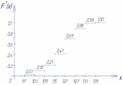 |
| Interval |  | 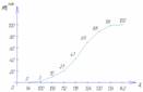 | 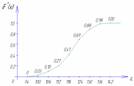 |
For graphic display variation series the most commonly used are polygon, histogram, cumulative curve, and empirical distribution function.
Table 2.3 (Grouping of the population of Russia by average per capita income in April 1994) is presented interval variation series.
It is convenient to analyze distribution series with the help of a graphic image, which makes it possible to judge the shape of the distribution. A clear idea of the nature of the change in the frequencies of the variation series is given by polygon and histogram.
The polygon is used when displaying discrete variation series.
Let's depict, for example, graphically the distribution of the housing stock by type of apartments (Table 2.10).
Table 2.10 - Distribution of the housing stock of the urban area by type of apartments (arbitrary numbers).

Rice. Housing stock allocation polygon
On the ordinate axis, not only the values of frequencies, but also the frequencies of the variation series can be plotted.
The histogram is taken for the image of the interval variation series... When constructing a histogram, the values of the intervals are plotted on the abscissa axis, and the frequencies are depicted by rectangles built at the corresponding intervals. The height of the bars in the case of equal spacing should be proportional to the frequencies. A histogram is a graph in which a series is shown in the form of bars adjacent to each other.
Let us graphically depict the interval distribution series given in table. 2.11.
Table 2.11 - Distribution of families by the size of living space per person (arbitrary numbers).
| N p / p | Groups of families according to the size of living space per person | The number of families with a given size of living space | Accumulated number of families |
| 1 | 3 – 5 | 10 | 10 |
| 2 | 5 – 7 | 20 | 30 |
| 3 | 7 – 9 | 40 | 70 |
| 4 | 9 – 11 | 30 | 100 |
| 5 | 11 – 13 | 15 | 115 |
| TOTAL | 115 | ---- | |

Rice. 2.2. Histogram of the distribution of families by the size of living space per person
Using the data of the accumulated series (Table 2.11), we construct cumulative distribution.

Rice. 2.3. Cumulative distribution of families by living space per person
The representation of the variation series in the form of cumulates is especially effective for variation series, the frequencies of which are expressed in fractions or percentages to the sum of the frequencies of the series.
If we change the axes when graphically depicting the variation series in the form of cumulates, then we get ogive... In fig. 2.4 shows the ogive built on the basis of the data in Table. 2.11.
A histogram can be converted to a distribution polygon by finding the midpoints of the sides of the rectangles and then connecting these points with straight lines. The resulting distribution polygon is shown in Fig. 2.2 with a dotted line.
When constructing a histogram of the distribution of the variation series with unequal intervals on the ordinate axis, not the frequencies are plotted, but the density of the feature distribution in the corresponding intervals.
The distribution density is the frequency calculated per unit interval width, i.e. how many units are in each group per unit of the interval. An example of calculating the distribution density is presented in table. 2.12.
Table 2.12 - Distribution of enterprises by the number of employees (conditional numbers)
| N p / p | Groups of enterprises by the number of employees, people | Number of enterprises | Interval size, persons | Distribution density |
| A | 1 | 2 | 3=1/2 | |
| 1 | Up to 20 | 15 | 20 | 0,75 |
| 2 | 20 – 80 | 27 | 60 | 0,25 |
| 3 | 80 – 150 | 35 | 70 | 0,5 |
| 4 | 150 – 300 | 60 | 150 | 0,4 |
| 5 | 300 – 500 | 10 | 200 | 0,05 |
| TOTAL | 147 | ---- | ---- |
For graphical representation of the variation series can also be used cumulative curve... With the help of cumulates (sum curve), a series of accumulated frequencies is displayed. The accumulated frequencies are determined by sequentially summing up the frequencies by groups and show how many units of the population have a characteristic value no greater than the considered value.

Rice. 2.4. Range of distribution of families by the size of living space per person
When constructing the cumulates of the interval variation series, the variants of the series are plotted along the abscissa axis, and the accumulated frequencies are plotted along the ordinate axis.
The set of values of the parameter studied in a given experiment or observation, ranked in magnitude (increase or decrease), is called the variation series.
Suppose that we measured blood pressure in ten patients in order to obtain an upper blood pressure threshold: systolic pressure, i.e. just one number.
Let us imagine that a series of observations (statistical aggregate) of arterial systolic pressure in 10 observations has the following form (Table 1):
Table 1
The components of the variation series are called variants. Variants represent the numerical value of the trait under study.
The construction of a variation series from a statistical population of observations is only the first step towards understanding the characteristics of the entire population. Next, it is necessary to determine the average level of the studied quantitative trait (average level of blood protein, average weight of patients, average time of onset of anesthesia, etc.)
The average level is measured using criteria called averages. The average value is a generalizing numerical characteristic of qualitatively homogeneous values, which characterizes the entire statistical population with one number according to one attribute. The average value expresses the general that is characteristic of a feature in a given set of observations.
Commonly used are three types of averages: mode (), median () and arithmetic mean ().
To determine any average value, it is necessary to use the results of individual observations, recording them in the form of a variation series (Table 2).
Fashion- the value that occurs most frequently in a series of observations. In our example, mode = 120. If there are no repeated values in the variation series, then the mode is said to be absent. If several values are repeated the same number of times, then the smallest of them is taken as the mode.
Median- the value that divides the distribution into two equal parts, the central or median value of a series of observations, ordered in ascending or descending order. So, if there are 5 values in the variation series, then its median is equal to the third term of the variation series, if there is an even number of members in the series, then the median is the arithmetic mean of its two central observations, i.e. if there are 10 observations in a row, then the median is equal to the arithmetic mean of 5 and 6 observations. In our example.
Note an important feature of the mode and median: their values are not influenced by the numerical values of the extreme variants.
Arithmetic mean calculated by the formula:
where is the observed value in the -th observation, and is the number of observations. For our case.
The arithmetic mean has three properties:
The middle one takes the middle position in the variation series. In a strictly symmetrical row.
The average is a generalizing value and for the average random fluctuations, differences in individual data are not visible. It reflects what is typical for the whole population.
The sum of deviations of all variants from the average is equal to zero:. The deviation of the variant from the mean is indicated.
The variation series consists of a variant and the corresponding frequencies. Of the ten obtained values, the number 120 occurred 6 times, 115 - 3 times, 125 - 1 time. Frequency () - the absolute number of individual variants in the aggregate, indicating how many times a given variant occurs in the variation series.
The variation series can be simple (frequency = 1) or grouped shortened, 3-5 options. A simple series is used with a small number of observations (), a grouped one - with a large number of observations ().
As a result of mastering this chapter, the student must: know
- indicators of variation and their relationship;
- basic laws of feature distribution;
- the essence of the consent criteria; be able to
- calculate indicators of variation and goodness-of-fit criteria;
- define characteristics of distributions;
- to evaluate the main numerical characteristics of statistical distribution series;
own
- methods of statistical analysis of distribution series;
- the basics of analysis of variance;
- methods of checking statistical distribution series for compliance with the basic distribution laws.
Variation indicators
In the statistical study of the characteristics of various statistical populations, it is of great interest to study the variation of the character of individual statistical units of the population, as well as the nature of the distribution of units for this characteristic. Variation - these are differences in the individual values of a trait in units of the studied population. The study of variation is of great practical importance. By the degree of variation, one can judge the boundaries of variation of a trait, the homogeneity of the population for this trait, the typicality of the average, the relationship of the factors that determine the variation. Variation indicators are used to characterize and order statistical populations.
The results of the summary and grouping of statistical observation materials, drawn up in the form of statistical distribution series, represent an ordered distribution of units of the studied population into groups according to the grouping (varying) attribute. If a qualitative feature is taken as the basis for the grouping, then such a distribution series is called attributive(distribution by profession, gender, color, etc.). If a distribution series is built on a quantitative basis, then such a series is called variational(distribution by height, weight, size wages etc.). Constructing a variation series means ordering the quantitative distribution of population units according to the values of the attribute, counting the number of population units with these values (frequency), and placing the results in a table.
Instead of the frequency of the variant, it is possible to apply its relation to the total volume of observations, which is called the frequency (relative frequency).
There are two types of variation series: discrete and interval. Discrete series - it is a variation series based on features with discontinuous change (discrete features). The latter include the number of employees in the enterprise, tariff category, the number of children in the family, etc. A discrete variation series is a table that consists of two graphs. The first column indicates the specific value of the attribute, and the second - the number of units of the population with a specific value of the attribute. If the attribute has a continuous change (the amount of income, work experience, the cost of fixed assets of the enterprise, etc., which, within certain limits, can take any values), then for this attribute it is possible to construct interval variation series. When constructing an interval variation series, the table also has two columns. The first contains the value of the feature in the interval "from - to" (options), the second - the number of units included in the interval (frequency). Frequency (repetition rate) - the number of repetitions of a separate variant of the attribute values. The intervals can be closed and open. Closed intervals are limited on both sides, i.e. have a border both lower ("from") and upper ("to"). Open intervals have any one border: either upper or lower. If the options are arranged in ascending or descending order, then the rows are called ranked.
For variation series, there are two types of frequency response options: accumulated frequency and accumulated frequency. The accumulated frequency shows how many observations the value of the feature took on values less than the specified one. The accumulated frequency is determined by summing the values of the frequency of the attribute for this group with all the frequencies of the previous groups. The accumulated frequency characterizes the proportion of observation units for which the values of the trait do not exceed the upper limit of the day group. Thus, the cumulative frequency shows the specific gravity of the variant in the aggregate, having a value not more than a given one. Frequency, frequency, absolute and relative density, accumulated frequency and frequency are characteristics of the magnitude of the variant.
Variations in the attribute of statistical units of the population, as well as the nature of the distribution, are studied using indicators and characteristics of the variation series, which include the average level of the series, the average linear deviation, the standard deviation, variance, coefficients of oscillation, variation, asymmetry, kurtosis, etc.
Average values are used to characterize the center of distribution. The average is a generalizing statistical characteristic in which the typical level of the trait that the members of the studied population possess is quantified. However, cases of coincidence of arithmetic means are possible with a different nature of the distribution, therefore, as the statistical characteristics of the variation series, the so-called structural averages are calculated - mode, median, as well as quantiles that divide the distribution series into equal parts (quartiles, deciles, percentiles, etc.) ).
Fashion - this is the value of a characteristic that occurs in a distribution series more often than its other values. For discrete series, this is the option with the highest frequency. In interval variation series, in order to determine the mode, it is necessary to determine, first of all, the interval in which it is located, the so-called modal interval. In a variation series with equal intervals, the modal interval is determined by the highest frequency, in series with unequal intervals - but the highest distribution density. Then, to determine the mode in rows with equal intervals, use the formula
where Mo is the value of the mode; x Mo is the lower boundary of the modal interval; h - the width of the modal interval; / Mo is the frequency of the modal interval; / Mo j is the frequency of the pre-modal interval; / Mo + 1 is the frequency of the post-modal interval, and for a series with unequal intervals in this calculation formula instead of the frequencies / Mo, / Mo, / Mo, distribution densities should be used Mind 0 _| , Mind 0> UMo + "
If there is a single mode, then the probability distribution random variable called unimodal; if there is more than one mode, it is called multimodal (polymodal, multimodal), in the case of two modes - bimodal. As a rule, multimodality indicates that the studied distribution does not obey the law normal distribution... For homogeneous populations, as a rule, unimodal distributions are characteristic. Multi-vertex also indicates the heterogeneity of the studied population. The appearance of two or more vertices makes it necessary to regroup the data in order to select more homogeneous groups.
In an interval variation series, the mode can be determined graphically using a histogram. For this, two intersecting lines are drawn from the top points of the highest column of the histogram to the top points of two adjacent columns. Then, from the point of their intersection, a perpendicular is lowered onto the abscissa axis. The value of the feature on the abscissa axis corresponding to the perpendicular is the mode. In many cases, when characterizing the population, fashion is preferred over the arithmetic mean as a generalized indicator.
Median - this is the central meaning of the feature; it is possessed by the central member of the ranked distribution series. In discrete series, in order to find the value of the median, its ordinal number is first determined. For this, when not even number units to the sum of all frequencies, one is added, the number is divided by two. If the number of units is even, there will be two median units in the series, therefore, in this case, the median is determined as the average of the values of the two median units. Thus, the median in a discrete variation series is the value that divides the series into two parts containing the same number options.
In the interval series, after determining the ordinal number of the median, the medial interval is found by the accumulated frequencies (parts), and then, using the formula for calculating the median, the value of the median itself is determined:

where Me is the median value; x Me - lower border of the median interval; h - the width of the median interval; - the sum of the frequencies of the distribution series; / D - accumulated frequency of the pre-median interval; / Me is the frequency of the median interval.
The median can be found graphically using the cumulate. For this, on the scale of accumulated frequencies (frequencies) of the cumulates from the point corresponding to the ordinal number of the median, a straight line is drawn parallel to the abscissa axis until it intersects with the cumulate. Further, from the point of intersection of the specified straight line with the cumulative, a perpendicular is lowered onto the abscissa axis. The value of a feature on the abscissa axis corresponding to the drawn ordinate (perpendicular) is the median.
The median is characterized by the following properties.
- 1. It does not depend on those values of the characteristic that are located on either side of it.
- 2. It has the property of minimality, which consists in the fact that the sum of the absolute deviations of the values of the attribute from the median is the minimum value in comparison with the deviation of the values of the attribute from any other value.
- 3. When combining two distributions with known medians, it is impossible to predict in advance the value of the median of the new distribution.
These properties of the median are widely used in designing point layouts. queuing- schools, clinics, gas stations, standpipes, etc. For example, if it is planned to build a polyclinic in a certain quarter of the city, then it is more expedient to locate it at a point in the quarter that divides in half not the length of the quarter, but the number of inhabitants.
The ratio of the mode, the median and the arithmetic mean indicates the nature of the distribution of the attribute in the aggregate, allows you to evaluate the symmetry of the distribution. If x Me then there is a right-sided asymmetry of the row. With a normal distribution NS - Me - Mo.
K. Pearson Based Alignment different types curves determined that for moderately asymmetric distributions, the following approximate relations between the arithmetic mean, median and mode are valid:

where Me is the median value; Mo is the meaning of fashion; x arithm - the value of the arithmetic mean.
If it becomes necessary to study the structure of the variation series in more detail, then the values of the feature are calculated, similar to the median. Such values of the characteristic divide all distribution units into equal numbers, they are called quantiles or gradients. Quantiles are subdivided into quartiles, deciles, percentiles, etc.
Quartiles divide the population into four equal parts. The first quartile is calculated similarly to the median using the formula for calculating the first quartile, having previously determined the first quarterly interval:

where Qi is the value of the first quartile; x Q ^ - lower border of the first quartile interval; h- the width of the first quarterly interval; /, - frequencies of the interval series;
Accumulated frequency in the interval preceding the first quartile interval; Jq (is the frequency of the first quartile interval.
The first quartile shows that 25% of population units are less than its value, and 75% - more. The second quartile is equal to the median, i.e. Q 2 = Me.
By analogy, the third quartile is calculated, having previously found the third quarterly interval:

where is the lower border of the third quartile interval; h- the width of the third quartile interval; /, - frequencies of the interval series; / X "- accumulated frequency in the interval preceding
G
third quartile interval; Jq is the frequency of the third quartile interval.
The third quartile shows that 75% of population units are less than its value, and 25% - more.
The difference between the third and first quartiles is the interquartile range:

where Aq is the value of the interquartile range; Q 3 - the value of the third quartile; Q, is the value of the first quartile.
Deciles divide the totality into 10 equal parts. A decile is such a value of a trait in a distribution series, which corresponds to tenths of the population size. By analogy with quartiles, the first decile shows that 10% of the population units are less than its value, and 90% - more, and the ninth decile reveals that 90% of the population units are less than its value, and 10% - more. The ratio of the ninth and first deciles, i.e. The decile coefficient is widely used in the study of income differentiation to measure the ratio of the income levels of the 10% richest and 10% of the poorest population. The percentiles divide the ranked population into 100 equal parts. The calculation, meaning and application of percentiles are similar to deciles.
Quartiles, deciles and other structural characteristics can be determined graphically by analogy with the median using cumulates.
The following indicators are used to measure the size of the variation: range of variation, mean linear deviation, standard deviation, variance. The magnitude of the variation range entirely depends on the randomness of the distribution of the extreme terms of the series. This indicator is of interest in cases where it is important to know what is the amplitude of fluctuations in the values of the attribute:

where R - the value of the range of variation; x max is the maximum value of the feature; x tt - the minimum value of the feature.
When calculating the range of variation, the value of the overwhelming majority of the members of the series is not taken into account, while the variation is associated with each value of the member of the series. This drawback is devoid of indicators, which are averages obtained from the deviations of individual values of a trait from their mean: the average linear deviation and the standard deviation. There is a direct relationship between individual deviations from the average and the variability of a particular trait. The stronger the fluctuation, the greater the absolute size of the deviations from the average.
The average linear deviation is the arithmetic mean of the absolute values of deviations of individual options from their mean.
Average linear deviation for ungrouped data

where / pr is the value of the average linear deviation; x, - is the value of the feature; NS - NS - the number of units in the population.
Average linear deviation of the grouped series

where / vz - the value of the average linear deviation; x, is the value of the feature; NS - the average value of the trait for the studied population; / is the number of population units in a separate group.
In this case, the signs of deviations are ignored, otherwise the sum of all deviations will be equal to zero. The average linear deviation, depending on the grouping of the analyzed data, is calculated using various formulas: for grouped and non-aggregated data. The average linear deviation, due to its conventionality, separately from other indicators of variation, is used in practice relatively rarely (in particular, to characterize the fulfillment of contractual obligations in terms of uniformity of delivery; in the analysis of foreign trade turnover, the composition of employees, the rhythm of production, product quality, taking into account technological features production, etc.).
The standard deviation characterizes how much, on average, the individual values of the trait under study deviate from the average value for the population, and is expressed in units of measurement of the trait under study. The standard deviation, being one of the main measures of variation, is widely used in assessing the boundaries of variation of a trait in a homogeneous population, in determining the values of the ordinates of the normal distribution curve, as well as in calculations related to organizing sample observation and establishing the accuracy of sample characteristics. The root-mean-square deviation of non-coarse data is calculated according to the following algorithm: each deviation from the mean is squared, all the squares are summed, after which the sum of the squares is divided by the number of members of the series and the square root is extracted from the quotient:

where a Iip is the mean standard deviation; Xj - the value of the feature; NS- the average value of the trait for the studied population; NS - the number of units in the population.
For grouped analyzed data, the standard deviation of the data is calculated using the weighted formula 
where - the value of the standard deviation; Xj - the value of the feature; NS - the average value of the trait for the studied population; f x - the number of population units in a particular group.
The expression under the root in both cases is called variance. Thus, the variance is calculated as the mean square of the deviations of the feature values from their mean. For unweighted (simple) values of the characteristic, the variance is determined as follows:

For weighted characteristic values

There is also a special simplified way of calculating variance: in general form 
for unweighted (simple) characteristic values  for weighted characteristic values
  using the conditional zero counting method

where a 2 is the value of the variance; x, - is the value of the feature; NS - average value of a feature, h - group interval value, t 1 - weight (A =
Dispersion has an independent expression in statistics and is one of the most important indicators of variation. It is measured in units corresponding to the square of the units of measurement of the trait under study.
The dispersion has the following properties.
- 1. The variance of the constant is zero.
- 2. A decrease in all values of a feature by the same value A does not change the magnitude of the variance. This means that the mean square of deviations can be calculated not by the given values of the attribute, but by their deviations from some constant number.
- 3. Decrease in all values of the attribute in k times reduces the variance by k 2 times, and the standard deviation - in k times, i.e. all the values of the attribute can be divided by some constant number (say, by the value of the interval of the series), calculate the standard deviation, and then multiply it by a constant number.
- 4. If you calculate the mean square of deviations from any value And at differing to some extent from the arithmetic mean, then it will always be greater than the mean square of deviations calculated from the arithmetic mean. In this case, the mean square of deviations will be larger by a quite definite amount - by the square of the difference between the mean and this conventionally taken value.
A variation of an alternative attribute consists in the presence or absence of the studied property in the units of the population. Quantitatively, the variation of an alternative feature is expressed in two values: the presence of the studied property in a unit is indicated by a unit (1), and its absence by a zero (0). The fraction of units that have the property under study is denoted by P, and the fraction of units that do not have this property is denoted by G. Thus, the variance of an alternative feature is equal to the product of the fraction of units with this property (P) by the fraction of units that do not have this property. (G). Greatest variation of the population is achieved in cases when a part of the population, which is 50% of the total volume of the population, has a feature, and another part of the population, also equal to 50%, does not have this feature, while the variance reaches maximum value equal to 0.25, i.e. P = 0.5, G = 1 - P = 1 - 0.5 = 0.5 and o 2 = 0.5 0.5 = 0.25. The lower bound of this indicator is zero, which corresponds to a situation in which there is no aggregate variation. Practical use variance of an alternative feature consists in constructing confidence intervals when conducting selective observation.
The smaller the variance and standard deviation, the more homogeneous the population and the more typical the mean will be. In the practice of statistics, it is often necessary to compare the variations of various features. For example, it is interesting to compare variations in the age of workers and their qualifications, length of service and wages, cost and profit, length of service and labor productivity, etc. For such comparisons, the indicators of the absolute variability of characteristics are unsuitable: it is impossible to compare the variability of the length of service, expressed in years, with the variation in wages, expressed in rubles. To carry out such comparisons, as well as comparisons of the fluctuations of the same feature in several populations with different arithmetic means, variation indicators are used - the oscillation coefficient, linear coefficient variation and coefficient of variation, which show the measure of fluctuation of extreme values around the mean.
Oscillation coefficient:

where V R - value of the oscillation coefficient; R- the value of the range of variation; NS -
Linear coefficient of variation ".

where Vj - the value of the linear coefficient of variation; I - the value of the mean linear deviation; NS - the average value of the trait for the studied population.
The coefficient of variation:

where V a - the value of the coefficient of variation; a - the value of the standard deviation; NS - the average value of the trait for the studied population.
The oscillation coefficient is the percentage of the range of variation to the mean value of the trait under study, and the linear coefficient of variation is the ratio of the average linear deviation to the mean value of the trait under study, expressed as a percentage. The coefficient of variation is the percentage of the standard deviation to the mean of the trait being studied. As a relative value, expressed as a percentage, the coefficient of variation is used to compare the degree of variation of various features. The coefficient of variation is used to estimate the homogeneity of the statistical population. If the coefficient of variation is less than 33%, then the studied population is homogeneous, and the variation is weak. If the coefficient of variation is more than 33%, then the studied population is heterogeneous, the variation is strong, and the average value is atypical and cannot be used as a generalizing indicator of this population. In addition, the coefficients of variation are used to compare the variability of one trait in different populations. For example, to assess the variation in the length of service of employees at two enterprises. How more value coefficient, the more significant the variation of the feature.
Based on the calculated quartiles, it is also possible to calculate the relative indicator of quarterly variation using the formula
where Q 2 and
The interquartile range is determined by the formula
![]()
Quartile bias is used in place of the range to avoid the disadvantages of using extreme values:

For unequally interval variation series, the distribution density is also calculated. It is defined as the quotient of dividing the corresponding frequency or frequency by the value of the interval. In unequally spaced series, absolute and relative distribution densities are used. The absolute density of the distribution is the frequency per unit length of the interval. The relative density of distribution is the frequency per unit length of the interval.
All of the above is true for distribution series, the distribution law of which is well described by the normal distribution law or is close to it.
The grouping method also allows you to measure variation(variability, variability) of signs. With a relatively small number of population units, variation is measured based on the ranked series of units that make up the population. The row is called ranked, if the units are arranged in ascending (descending) order of the attribute.
However, the ranked series are rather poorly indicative when it is necessary Comparative characteristics variations. In addition, in many cases one has to deal with statistical populations consisting of a large number units that are practically difficult to represent in the form of a specific series. In this regard, for an initial general acquaintance with statistical data and especially to facilitate the study of variation in characteristics, the phenomena and processes under study are usually combined into groups, and the grouping results are drawn up in the form of group tables.
If there are only two columns in the group table - groups according to the selected feature (options) and the number of groups (frequency or frequency), it is called near distribution.
Distribution series - The simplest kind of structural grouping by one attribute, displayed in a group table with two columns, which contain the options and frequencies of the attribute. In many cases, with such a structural grouping, i.e. with the compilation of distribution series, the study of the initial statistical material begins.
A structural grouping in the form of a distribution series can be turned into a true structural grouping if the selected groups are characterized not only by frequencies, but also by other statistical indicators. The main purpose of the distribution series is to study the variation of features. The theory of distribution series is developed in detail by mathematical statistics.
The distribution series is divided by attributive(grouping according to attributive characteristics, for example, dividing the population by sex, nationality, marital status etc.) and variational(grouping by quantitative characteristics).
Variational series is a group table that contains two columns: the grouping of units according to one quantitative characteristic and the number of units in each group. The intervals in the variation series are usually equal and closed. The variation series is the following population grouping in Russia in terms of average per capita cash income(Table 3.10).
Table 3.10
Distribution of the population of Russia by average per capita income in 2004-2009
|
Population groups by average per capita money income, rubles / month |
Population in the group, in% of the total |
|||||
|
8 000,1-10 000,0 |
||||||
|
10 000,1-15 000,0 |
||||||
|
15 000,1-25 000,0 |
||||||
|
More than 25,000.0 |
||||||
|
All population |
||||||
Variational series, in turn, are subdivided into discrete and interval. Discrete Variational series combine variants of discrete features that vary within narrow limits. An example of a discrete variation series is the distribution of Russian families by the number of children they have.
Interval Variational series combine variants of either continuous features or discrete features varying over a wide range. The range of variation is the distribution of the population of Russia in terms of average per capita money income.
Discrete variational series are not used very often in practice. Meanwhile, their compilation is not difficult, since the composition of the groups is determined by the specific options that the studied grouping characteristics actually possess.
Interval variation series are more widespread. When they are drawn up, complex issue the number of groups, as well as the size of the intervals to be set.
The principles for solving this issue are set out in the chapter on the construction methodology. statistical groupings(see paragraph 3.3).
Variational series are a means of folding or compressing diverse information into a compact form, they can be used to make a fairly clear judgment about the nature of the variation, to study the differences in the features of the phenomena included in the studied set. But the most important value of the variation series is that on their basis special generalizing characteristics of variation are calculated (see Chapter 7).
(definition of the variation series; components of the variation series; three forms of the variation series; expediency of constructing an interval series; conclusions that can be drawn from the constructed series)
The variation series is the sequence of all the elements of the sample, arranged in a non-decreasing order. Identical elements are repeated
Variational ones are series built on a quantitative basis.
Variational distribution series consist of two elements: options and frequencies:
Variants are the numerical values of a quantitative characteristic in the variation series of the distribution. They can be positive and negative, absolute and relative. So, when grouping enterprises according to the results of economic activity, the positive options are profit, and negative numbers Is a loss.
Frequencies are the numbers of individual variants or each group of the variation series, i.e. these are numbers showing how often one or another variant occurs in a distribution series. The sum of all frequencies is called the volume of the population and is determined by the number of elements of the entire population.
Frequencies are frequencies expressed as relative values (fractions of units or percentages). The sum of the frequencies is equal to one or 100%. Replacing frequencies with frequencies allows one to compare the series of variations with a different number of observations.
There are three forms of the variation series: ranked range, discrete range and interval range.
A ranked series is the distribution of individual units of a population in ascending or descending order of the trait under study. Ranking allows you to easily divide quantitative data into groups, immediately find the smallest and largest values of a feature, highlight the values that are most often repeated.
Other forms of the variation series are group tables compiled according to the nature of the variation in the values of the trait under study. By the nature of the variation, discrete (discontinuous) and continuous signs are distinguished.
A discrete series is a variation series based on features with discontinuous change (discrete features). The latter include the wage rate, the number of children in the family, the number of employees at the enterprise, etc. These characteristics can only take on a finite number of specific values.
A discrete variation series is a table that consists of two graphs. The first column indicates the specific value of the attribute, and the second - the number of units of the population with a specific value of the attribute.
If a feature has a continuous change (the amount of income, work experience, the cost of fixed assets of the enterprise, etc., which within certain limits can take any values), then for this feature it is necessary to build an interval variation series.
The group table also has two columns here. The first contains the value of the feature in the interval "from - to" (options), the second - the number of units included in the interval (frequency).
Frequency (repetition rate) - the number of repetitions of a separate variant of the attribute values, denoted by fi, and the sum of frequencies equal to the volume of the studied population is denoted
Where k is the number of options for characteristic values
Very often, the table is supplemented with a column in which the accumulated frequencies S are calculated, which show how many units of the population have a feature value no more than a given value.
A discrete variation series of a distribution is a series in which groups are composed according to a feature that changes discretely and takes only integer values.
An interval variation series of a distribution is a series in which the grouping attribute that forms the basis of the grouping can take any values in a certain interval, including fractional ones.
An interval variation series is an ordered set of intervals of variation of the values of a random variable with the corresponding frequencies or frequencies of occurrence of values of the quantity in each of them.
Interval series It is advisable to construct distributions, first of all, with continuous variation of a feature, and also if discrete variation manifests itself in wide limits, i.e. the number of options for a discrete feature is large enough.
Several conclusions can already be drawn from this series. For example, the mean of the variation series (median) can be an estimate of the most likely measurement result. The first and last element of the variation series (i.e., the minimum and maximum sample unit) show the dispersion of the sample items. Sometimes if the first or last element is very different from the rest of the sample, then they are excluded from the measurement results, considering that these values were obtained as a result of some gross failure, for example, technology.