Solve the system of linear equations bx 0. System of linear equations
Solution we carry out with the help of a calculator. Let's write out the extended and basic matrices: 
The dotted line separates the main matrix A. Above we write the unknown systems, bearing in mind the possible rearrangement of the terms in the equations of the system. Determining the rank of the extended matrix, we simultaneously find the rank and the main one. In matrix B, the first and second columns are proportional. Of the two proportional columns, only one can fall into the basic minor, so we transfer, for example, the first column behind the dashed line with the opposite sign. For the system, this means moving the terms from x 1 to the right side of the equations. 
Let's bring the matrix to a triangular form. We will work only with rows, since multiplying a row of a matrix by a number other than zero and adding to another row for the system means multiplying the equation by the same number and adding it with another equation, which does not change the solution of the system. We work with the first row: multiply the first row of the matrix by (-3) and add to the second and third rows in turn. Then we multiply the first line by (-2) and add to the fourth. 
The second and third lines are proportional, therefore, one of them, for example the second, can be crossed out. This is tantamount to deleting the second equation of the system, since it is a consequence of the third. 
Now we are working with the second line: multiply it by (-1) and add to the third. 
The dashed minor has the highest order (of the possible minors) and is nonzero (it is equal to the product elements on the main diagonal), and this minor belongs to both the main matrix and the extended one, therefore, rangA = rangB = 3.
Minor  is basic. It includes the coefficients for the unknowns x 2, x 3, x 4, which means that the unknowns x 2, x 3, x 4 are dependent, and x 1, x 5 are free.
We transform the matrix, leaving only the base minor on the left (which corresponds to point 4 of the above solution algorithm). 
The system with the coefficients of this matrix is equivalent to the original system and has the form
Using the method of eliminating unknowns, we find: ![]() , ,
, ,
We got the ratios expressing the dependent variables x 2, x 3, x 4 through free x 1 and x 5, that is, we found a general solution: 
By assigning any values to the free unknowns, we obtain any number of particular solutions. Let's find two particular solutions:
1) let x 1 = x 5 = 0, then x 2 = 1, x 3 = -3, x 4 = 3;
2) put x 1 = 1, x 5 = -1, then x 2 = 4, x 3 = -7, x 4 = 7.
Thus, we found two solutions: (0.1, -3.3.0) - one solution, (1.4, -7.7, -1) - another solution.
Example 2... Investigate compatibility, find a general and one particular solution to the system 
Solution... We rearrange the first and second equations to have unity in the first equation and write the matrix B. 
We get zeros in the fourth column, operating on the first row: 
Now we get the zeros in the third column using the second row: 
 The third and fourth lines are proportional, so one of them can be crossed out without changing the rank:
We multiply the third row by (–2) and add to the fourth: 
We see that the ranks of the main and extended matrices are equal to 4, and the rank coincides with the number of unknowns, therefore, the system has only decision:
;
x 4 = 10 - 3x 1 - 3x 2 - 2x 3 = 11.
Example 3... Examine the system for compatibility and find a solution if it exists. 
Solution... We compose an extended matrix of the system. 
 We rearrange the first two equations so that there is 1 in the upper left corner:
Multiplying the first line by (-1), add it to the third: 
Multiply the second row by (-2) and add to the third: 
The system is inconsistent, since in the main matrix we got a row consisting of zeros, which is crossed out when the rank is found, and in the extended matrix the last row will remain, that is, r B> r A.
Exercise... Investigate this system of equations for consistency and solve it using matrix calculus.
Solution
Example... Prove system compatibility linear equations and solve it in two ways: 1) the Gauss method; 2) Cramer's method. (enter the answer in the form: x1, x2, x3)
Solution: doc: doc: xls
Answer: 2,-1,3.
Example... A system of linear equations is given. Prove its compatibility. Find a general solution to the system and one particular solution.
Solution
Answer: x 3 = - 1 + x 4 + x 5; x 2 = 1 - x 4; x 1 = 2 + x 4 - 3x 5
Exercise... Find general and specific solutions for each system.
Solution. Let us investigate this system using the Kronecker-Capelli theorem.
Let's write out the extended and basic matrices:
| 1 | 1 | 14 | 0 | 2 | 0 |
| 3 | 4 | 2 | 3 | 0 | 1 |
| 2 | 3 | -3 | 3 | -2 | 1 |
| x 1 | x 2 | x 3 | x 4 | x 5 |
Here matrix A is in bold.
Let's bring the matrix to a triangular form. We will work only with rows, since multiplying a row of a matrix by a number other than zero and adding to another row for the system means multiplying the equation by the same number and adding it with another equation, which does not change the solution of the system.
Multiply the 1st row by (3). Multiply the 2nd row by (-1). Let's add the 2nd line to the 1st:
| 0 | -1 | 40 | -3 | 6 | -1 |
| 3 | 4 | 2 | 3 | 0 | 1 |
| 2 | 3 | -3 | 3 | -2 | 1 |
Multiply the 2nd row by (2). Multiply the 3rd row by (-3). Let's add the 3rd line to the 2nd:
| 0 | -1 | 40 | -3 | 6 | -1 |
| 0 | -1 | 13 | -3 | 6 | -1 |
| 2 | 3 | -3 | 3 | -2 | 1 |
Multiply the 2nd row by (-1). Let's add the 2nd line to the 1st:
| 0 | 0 | 27 | 0 | 0 | 0 |
| 0 | -1 | 13 | -3 | 6 | -1 |
| 2 | 3 | -3 | 3 | -2 | 1 |
The highlighted minor has the highest order (of the possible minors) and is nonzero (it is equal to the product of the elements on the reverse diagonal), and this minor belongs to both the main matrix and the extended one, therefore, rang (A) = rang (B) = 3 . Since the rank of the main matrix is equal to the rank of the extended matrix, then the system is a joint.
This minor is basic. It includes the coefficients for the unknowns x 1, x 2, x 3, which means that the unknowns x 1, x 2, x 3 are dependent (basic), and x 4, x 5 are free.
We transform the matrix, leaving only the base minor on the left.
| 0 | 0 | 27 | 0 | 0 | 0 |
| 0 | -1 | 13 | -1 | 3 | -6 |
| 2 | 3 | -3 | 1 | -3 | 2 |
| x 1 | x 2 | x 3 | x 4 | x 5 |
27x 3 =
- x 2 + 13x 3 = - 1 + 3x 4 - 6x 5
2x 1 + 3x 2 - 3x 3 = 1 - 3x 4 + 2x 5
Using the method of eliminating unknowns, we find:
We obtained relations expressing the dependent variables x 1, x 2, x 3 through free x 4, x 5, that is, we found common decision:
x 3 = 0
x 2 = 1 - 3x 4 + 6x 5
x 1 = - 1 + 3x 4 - 8x 5
undefined since has more than one solution.
Exercise... Solve the system of equations.
Answer: x 2 = 2 - 1.67x 3 + 0.67x 4
x 1 = 5 - 3.67x 3 + 0.67x 4
By assigning any values to the free unknowns, we obtain any number of particular solutions. The system is undefined
The equation has a solution: if at least one of the coefficients of the unknowns is nonzero. In this case, any -dimensional vector is called a solution to the equation if, after substituting its coordinates, the equation turns into an identity.
General characteristics of the resolved system of equations
Example 20.1Describe the system of equations.
![]()
Solution:
1. Is there a conflicting equation in the composition?(If the coefficients, in this case the equation has the form: and is called contradictory.)
- If the system contains a contradictory, then such a system is incompatible and has no solution
2. Find All Allowed Variables. (Unknown is calledpermitted for a system of equations if it enters into one of the equations of the system with a coefficient of +1, and does not enter into the other equations (i.e., enters with a coefficient equal to zero).
3. Is the system of equations allowed? (The system of equations is called allowed if each equation of the system contains a resolved unknown, among which there are no coinciding ones)
In the general case, the resolved system of equations has the form:The allowed unknowns, taken one at a time from each equation of the system, form full set of resolved unknowns systems. (in our example it is)
The resolved unknowns included in the complete set are also called basic(), and not included in the set - free ().

At this stage, the main thing is to understand what is resolved unknown(included in the basis and free).
General Partial Basic Solution
By general decision An allowed system of equations is a set of expressions for the resolved unknowns in terms of free terms and free unknowns:

By private decision is called the solution obtained from the general for specific values of free variables and unknowns.
Basic solution is called a particular solution obtained from the general one at zero values of free variables.
- The basic solution (vector) is called degenerate if the number of its nonzero coordinates is less than the number of allowed unknowns.
- The basic solution is called non-degenerate if the number of its nonzero coordinates is equal to the number of allowed unknowns of the system included in the complete set.
Example 1. Find the general, basic and any particular solution of the system of equations:Theorem (1)
Allowed system of equations is always consistent(because it has at least one solution); and if the system has no free unknowns,(that is, in the system of equations, all allowed ones are included in the basis) then it is defined(has only one solution); if there is at least one free variable, then the system is undefined(has an infinite number of solutions).
![]()
Solution:
1. Checking if the system is legal?
- The system is resolved (since each of the equations contains a resolved unknown)
2. We include in the set the resolved unknowns - one from each equation.
3. We write down the general solution depending on which resolved unknowns we included in the set.

4. We find a particular solution... To do this, we equate free variables that we did not include in the set to equate to arbitrary numbers.
![]()
Answer: private solution(one of the options)
5. Finding the basic solution... To do this, we equate free variables that we did not include in the set to zero.
Elementary transformations of linear equations
Systems of linear equations are reduced to equivalent allowed systems using elementary transformations.
Theorem (2)
If any multiply the equation of the system by some nonzero number, and leave the rest of the equations unchanged, then. (that is, if you multiply the left and right sides of the equation by the same number, you get an equation equivalent to this one)
Theorem (3)
If to some equation of the system add another, and leave all other equations unchanged, then we get a system equivalent to the given... (that is, if you add two equations (adding their left and right sides), you get an equation equivalent to the data)
Corollary from Theorems (2 and 3)
If to some equation add another, multiplied by some number, and leave all other equations unchanged, then we get a system equivalent to the given.
Conversion formulas for system coefficients
If we have a system of equations and we want to transform it into a resolved system of equations, the Jordan-Gauss method will help us.
Jordan transform with a resolving element allows you to get the resolved unknown in the equation with a number for the system of equations. (example 2).
The Jordan transform consists of two types of elementary transformations:Let's say we want to make the unknown in the lower equation the resolved unknown. To do this, we must divide by, so that the amount.
Example 2 Let's recalculate the coefficients of the system
When dividing an equation with a number by, its coefficients are recalculated according to the formulas:
![]()
To eliminate from an equation with a number, you need to multiply the equation with a number by and add to this equation.
Theorem (4) On the reduction of the number of equations in the system.
If the system of equations contains a trivial equation, then it can be excluded from the system, and the resulting system is equivalent to the original one.
Theorem (5) On the incompatibility of a system of equations.
If a system of equations contains a contradictory equation, then it is inconsistent.
Algorithm of the Jordan-Gauss method
The algorithm for solving systems of equations by the Jordan-Gauss method consists of a number of steps of the same type, at each of which the actions are performed in the following order:
- Checks to see if the system is inconsistent. If the system contains a contradictory equation, then it is inconsistent.
- The possibility of reducing the number of equations is checked. If the system contains a trivial equation, it is deleted.
- If the system of equations is resolved, then the general solution of the system is written down and, if necessary, particular solutions.
- If the system is not resolved, then in the equation that does not contain the resolved unknown, a resolving element is selected and the Jordan transform is performed with this element.
- Then go to point 1 again.
Find: two general and two corresponding basic solutions

Solution:
The calculations are shown in the following table:
Actions on equations are shown to the right of the table. The arrows show to which equation the equation with the resolving element is added, multiplied by a suitable factor.

The first three rows of the table contain the coefficients for the unknowns and the right-hand sides of the original system. The results of the first Jordan transform with the resolving element equal to one are shown in lines 4, 5, 6. The results of the second Jordan transform with the resolving element equal to (-1) are given in lines 7, 8, 9. Since the third equation is trivial, it can be consider.
We continue to deal with systems of linear equations. So far, we have looked at systems that have a single solution. Such systems can be solved in any way: substitution method("School"), by Cramer's formulas, matrix method, Gaussian method... However, in practice, two more cases are widespread when:
1) the system is incompatible (has no solutions);
2) the system has infinitely many solutions.
For these systems, the most universal of all solution methods is used - Gauss method... In fact, the "school" method will lead to the answer, but in higher mathematics it is customary to use the Gaussian method of successive elimination of unknowns. For those who are not familiar with the Gaussian method algorithm, please study the lesson first Gauss method
The elementary matrix transformations themselves are exactly the same, the difference will be in the end of the solution. Let's first consider a couple of examples when the system has no solutions (inconsistent).
Example 1
What immediately catches the eye in this system? The number of equations is less than the number of variables. There is a theorem that states: "If the number of equations in the system is less than the number of variables, then the system is either inconsistent or has infinitely many solutions. " And it remains only to find out.
The beginning of the solution is completely ordinary - we write down the extended matrix of the system and, using elementary transformations, bring it to a stepwise form:

(1). On the top left step, we need to get (+1) or (–1). There are no such numbers in the first column, so rearranging the rows will give nothing. The unit will have to be organized independently, and this can be done in several ways. We did this. To the first line add the third line multiplied by (–1).
(2). Now we get two zeros in the first column. To the second line we add the first line multiplied by 3. To the third line we add the first line multiplied by 5.
(3). After the performed transformation, it is always advisable to look, and is it possible to simplify the resulting lines? Can. Divide the second row by 2, at the same time getting the desired (–1) on the second step. Divide the third row by (–3).
(4). Add the second line to the third line. Probably everyone paid attention to the bad line that turned out as a result of elementary transformations:
![]() ... It is clear that this cannot be so.
... It is clear that this cannot be so.
Indeed, we rewrite the resulting matrix

back to the system of linear equations:

If, as a result of elementary transformations, a string of the form , whereλ - a number other than zero, then the system is incompatible (has no solutions).
How do I record the ending of an assignment? You must write down the phrase:
“As a result of elementary transformations, a string of the form was obtained, where λ ≠ 0 ". Answer: "The system has no solutions (inconsistent)."
Please note that in this case there is no backtracking of the Gaussian algorithm, there are no solutions and there is simply nothing to find.
Example 2
Solve a system of linear equations 
This is an example for independent decision. Complete solution and the answer at the end of the lesson.
Again, we remind you that your decision course may differ from our decision course, the Gauss method does not specify an unambiguous algorithm, you have to guess about the order of actions and the actions themselves in each case independently.
Another one technical feature solutions: elementary transformations can be stopped immediately, as soon as a line of the form appeared, where λ ≠ 0 ... Consider conditional example: suppose that after the first transformation the matrix is obtained
 .
.
This matrix has not yet been reduced to a stepped form, but there is no need for further elementary transformations, since a line of the form has appeared, where λ ≠ 0 ... You should immediately answer that the system is incompatible.
When a system of linear equations has no solutions, this is almost a gift to the student, since a short solution is obtained, sometimes literally in 2-3 steps. But everything in this world is balanced, and the problem in which the system has infinitely many solutions is just longer.
Example 3:
Solve a system of linear equations

There are 4 equations and 4 unknowns, so the system can either have a single solution, or have no solutions, or have infinitely many solutions. Be that as it may, but the Gauss method will lead us to the answer anyway. This is its versatility.
The beginning is again standard. Let us write down the extended matrix of the system and, using elementary transformations, bring it to a stepwise form:

That's all, and you were afraid.
(1). Please note that all the numbers in the first column are divisible by 2, so we are satisfied with two on the upper left step. To the second line add the first line multiplied by (–4). To the third line add the first line multiplied by (–2). To the fourth line add the first line multiplied by (–1).
Attention! Many may be tempted from the fourth line subtract first line. This can be done, but it is not necessary, experience shows that the probability of an error in calculations increases several times. Just add: to the fourth line add the first line multiplied by (–1) - exactly!
(2). The last three lines are proportional, two of them can be deleted. Here again you need to show increased attention, but are the lines really proportional? To be on the safe side, it will not be superfluous to multiply the second line by (–1), and divide the fourth line by 2, resulting in three identical lines. And only then delete two of them. As a result of elementary transformations, the expanded matrix of the system is reduced to a stepwise form:

When filling out a task in a notebook, it is advisable to make the same notes in pencil for clarity.
Let's rewrite the corresponding system of equations: 
The only solution of the system here does not smell like "usual". A bad line where λ ≠ 0, also no. This means that this is the third remaining case - the system has infinitely many solutions.
The infinite number of solutions to the system are briefly written in the form of the so-called overall system solution.
Common decision we find the systems using the reverse course of the Gauss method. For systems of equations with an infinite set of solutions, new concepts appear: "Basic variables" and "Free variables"... First, let's define which variables we have basic, and which variables - free... It is not necessary to explain in detail the terms of linear algebra, it is enough to remember that there are such basic variables and free variables.
Basic variables always "sit" strictly on the steps of the matrix... V this example basic variables are x 1 and x 3 .
Free variables are everything remaining variables that did not get a rung. In our case, there are two of them: x 2 and x 4 - free variables.
Now you need allbasic variables to express only throughfree variables... The reverse of the Gaussian algorithm traditionally works from the bottom up. From the second equation of the system, we express the basic variable x 3:
Now let's look at the first equation: ![]() ... First, we substitute the found expression into it:
... First, we substitute the found expression into it:
![]()
It remains to express the basic variable x 1 via free variables x 2 and x 4:

In the end, we got what we need - all basic variables ( x 1 and x 3) expressed only through free variables ( x 2 and x 4):
![]()
Actually, the general solution is ready:
![]() .
.
How to write down the general solution correctly? First of all, free variables are written into the general solution "by themselves" and strictly in their places. In this case, free variables x 2 and x 4 should be written in the second and fourth positions:
 .
.
The obtained expressions for the basic variables ![]() and, obviously, you need to write in the first and third positions:
and, obviously, you need to write in the first and third positions:

From the general solution of the system, you can find infinitely many private solutions... It’s very simple. Free variables x 2 and x 4 are called so because they can be given any end values... The most popular values are zero, because this is the simplest solution to the particular solution.
Substituting ( x 2 = 0; x 4 = 0) into the general solution, we get one of the particular solutions:
![]() , or is a particular solution corresponding to free variables at values ( x 2 = 0; x 4 = 0).
, or is a particular solution corresponding to free variables at values ( x 2 = 0; x 4 = 0).
Units are another sweet couple, substitute ( x 2 = 1 and x 4 = 1) into a general solution:
![]() , i.e. (-1; 1; 1; 1) is another particular solution.
, i.e. (-1; 1; 1; 1) is another particular solution.
It is easy to see that the system of equations has infinitely many solutions, since we can give free variables any values.
Each the particular solution must satisfy to each equation of the system. This is the basis for the "quick" check of the correctness of the solution. Take, for example, a particular solution (-1; 1; 1; 1) and substitute it into the left side of each equation of the original system:
Everything should fit together. And with any particular decision you receive - everything should also agree.
Strictly speaking, checking a particular solution sometimes deceives, i.e. some particular solution may satisfy each equation of the system, but the general solution itself is actually found incorrectly. Therefore, first of all, the check of the general solution is more thorough and reliable.
How to check the resulting general solution ![]() ?
?
It is not difficult, but it requires a lot of time-consuming transformations. You need to take expressions basic variables, in this case ![]() and, and substitute them in the left side of each equation of the system.
and, and substitute them in the left side of each equation of the system.
On the left side of the first equation of the system:

Received right part the original first equation of the system.
On the left side of the second equation of the system:

The right-hand side of the original second equation of the system is obtained.
And further - to the left-hand sides of the third and fourth equations of the system. This check takes longer, but it guarantees one hundred percent correctness of the overall solution. In addition, in some tasks, it is precisely the verification of the general solution that is required.
Example 4:
Solve the system by the Gaussian method. Find a general solution and two particular ones. Check the general solution.

This is an example for a do-it-yourself solution. Here, by the way, again the number of equations is less than the number of unknowns, which means that it is immediately clear that the system will be either incompatible or with an infinite set of solutions.
Example 5:
Solve a system of linear equations. If the system has infinitely many solutions, find two particular solutions and check the general solution

Solution: Let us write down the extended matrix of the system and, using elementary transformations, bring it to a stepwise form:

(1). Add the first line to the second line. To the third line we add the first line multiplied by 2. To the fourth line we add the first line multiplied by 3.
(2). To the third line, add the second line multiplied by (–5). To the fourth line, add the second line multiplied by (–7).
(3). The third and fourth lines are the same, we delete one of them. Here is such beauty:

Basic variables sit on rungs, therefore basic variables.
There is only one free variable that did not get a step here:.
(4). Reverse move. Let's express the basic variables in terms of a free variable:
From the third equation:
![]()
Consider the second equation and substitute the found expression into it:
![]() ,
, ![]() , ,
, ,
Consider the first equation and substitute the found expressions and into it:

Thus, the general solution for one free variable is x 4:
![]()
Once again, how did it come about? Free variable x 4 sits alone in its rightful fourth place. The resulting expressions for the basic variables are also in their places.
Let's check the general solution right away.
We substitute the basic variables,, in the left side of each equation of the system:


The corresponding right-hand sides of the equations are obtained, thus, the correct general solution is found.
Now from the found common solution ![]() we get two particular solutions. All variables are expressed here through a single free variable x 4 . You don't need to rack your brains.
we get two particular solutions. All variables are expressed here through a single free variable x 4 . You don't need to rack your brains.
Let be x 4 = 0, then ![]() - the first particular solution.
- the first particular solution.
Let be x 4 = 1, then ![]() - one more particular solution.
- one more particular solution.
Answer: Common decision: ![]() ... Private solutions:
... Private solutions:
![]() and .
and .
Example 6:
Find the general solution of a system of linear equations.

We have already checked the general decision, the answer can be trusted. Your course of decision may differ from our course of decision. The main thing is for common decisions to coincide. Probably, many have noticed an unpleasant moment in the solutions: very often, during the reverse course of the Gauss method, we had to tinker with ordinary fractions... In practice, this is true, cases when there are no fractions are much less common. Be prepared mentally, and most importantly, technically.
Let us dwell on the features of the solution that were not found in the solved examples. The general solution of the system can sometimes include a constant (or constants).
For example, the general solution is:. Here one of the basic variables is equal to a constant number:. There is nothing exotic in this, it happens. Obviously, in this case, any particular solution will contain an A in the first position.
Rarely, but there are systems in which number of equations more quantity variables... However, the Gauss method works under the harshest conditions. It is necessary to calmly reduce the expanded matrix of the system to a stepped form according to the standard algorithm. Such a system can be inconsistent, it can have infinitely many solutions, and, oddly enough, it can have a single solution.
Let's repeat in our advice - in order to feel comfortable when solving a system using the Gaussian method, you should fill your hand and solve at least a dozen systems.
Solutions and Answers:
Example 2:
Solution:Let us write down the extended matrix of the system and, using elementary transformations, bring it to a stepwise form.
Elementary transformations performed:
(1) The first and third lines are reversed.
(2) The first line multiplied by (–6) was added to the second line. The first line multiplied by (–7) was added to the third line.
(3) The second line multiplied by (–1) was added to the third line.
As a result of elementary transformations, a string of the form, where λ ≠ 0 .This means that the system is incompatible.Answer: no solutions.
Example 4:
Solution:Let us write down the extended matrix of the system and, using elementary transformations, bring it to a stepwise form:

Conversions performed:
(1). The first line multiplied by 2 was added to the second line. The first line multiplied by 3 was added to the third line.
There is no one for the second step , and transformation (2) is aimed at obtaining it.
(2). The third line was added to the second line multiplied by –3.
(3). The second and third lines were swapped (rearranged the resulting -1 to the second step)
(4). The third line was added to the second line multiplied by 3.
(5). The sign of the first two lines was changed (multiplied by –1), the third line was divided by 14.
Reverse:
(1). Here - basic variables (which are on the steps), and - free variables (who did not get a step).
(2). Let's express the basic variables in terms of free variables:
From the third equation: .
(3). Consider the second equation:, particular solutions:
Answer: Common decision: ![]()
Complex numbers
In this section, we will get acquainted with the concept complex number, consider algebraic, trigonometric and exemplary form complex number. We will also learn how to perform actions with complex numbers: addition, subtraction, multiplication, division, exponentiation and root extraction.
To master complex numbers, you do not need any special knowledge from the course higher mathematics, and the material is available even to a student. It is enough to be able to perform algebraic operations with "ordinary" numbers, and remember trigonometry.
First, let's remember the "ordinary" Numbers. In mathematics, they are called set of real numbers and denoted by the letter R, or R (thickened). All real numbers sit on the familiar number line:

The company of real numbers is very variegated - here there are integers, fractions, and irrational numbers. In this case, each point of the numerical axis necessarily corresponds to a certain real number.
Gauss's method, also called the method of successive elimination of unknowns, is as follows. With the help of elementary transformations, the system of linear equations is brought to such a form that its matrix of coefficients turns out to be trapezoidal (same as triangular or stepped) or close to trapezoidal (direct move of the Gauss method, further - just a direct move). An example of such a system and its solution is in the figure above.
In such a system, the last equation contains only one variable and its value can be found unambiguously. Then the value of this variable is substituted into the previous equation ( reverse Gauss method , then just reverse), from which the previous variable is found, and so on.
In a trapezoidal (triangular) system, as we see, the third equation no longer contains the variables y and x, and the second equation is the variable x .
After the matrix of the system has taken a trapezoidal shape, it is no longer difficult to understand the question of the compatibility of the system, determine the number of solutions and find the solutions themselves.
The advantages of the method:
- when solving systems of linear equations with the number of equations and unknowns more than three, the Gauss method is not as cumbersome as the Cramer method, since less calculations are required when solving the Gauss method;
- using the Gauss method, one can solve indefinite systems of linear equations, that is, having a general solution (and we will analyze them in this lesson), and using Cramer's method, one can only state that the system is indefinite;
- you can solve systems of linear equations in which the number of unknowns is not equal to the number of equations (we will also analyze them in this lesson);
- the method is based on elementary (school) methods - the method of substitution of unknowns and the method of adding equations, which we touched upon in the corresponding article.
So that everyone is imbued with the simplicity with which trapezoidal (triangular, stepwise) systems of linear equations are solved, we will give a solution to such a system using the reverse motion. A quick solution to this system was shown in the picture at the beginning of the lesson.
Example 1. Solve a system of linear equations using the reverse motion:

Solution. In this trapezoidal system, the variable z is uniquely found from the third equation. We substitute its value into the second equation and get the value by the variable y:
Now we know the values of two variables - z and y... We substitute them into the first equation and get the value of the variable x:
From the previous steps, we write out the solution to the system of equations:
![]()
To obtain such a trapezoidal system of linear equations, which we solved very simply, it is required to apply a direct move associated with elementary transformations of the system of linear equations. It is also not very difficult.
Elementary transformations of a system of linear equations
Repeating the school method of algebraic addition of the equations of the system, we found out that another equation of the system can be added to one of the equations of the system, and each of the equations can be multiplied by some numbers. As a result, we obtain a system of linear equations equivalent to the given one. In it, one equation already contained only one variable, substituting the value of which into other equations, we arrive at a solution. Such addition is one of the types of elementary transformation of the system. When using the Gaussian method, we can use several types of transformations.

The animation above shows how the system of equations gradually turns into a trapezoidal one. That is, one that you saw in the very first animation and made sure for yourself that it is easy to find the values of all unknowns from it. How to perform such a transformation and, of course, examples will be discussed further.
When solving systems of linear equations with any number of equations and unknowns in the system of equations and in the extended matrix of the system can:
- rearrange the lines (this was mentioned at the very beginning of this article);
- if, as a result of other transformations, equal or proportional rows appeared, they can be deleted, except for one;
- delete "zero" lines where all coefficients are equal to zero;
- any string to multiply or divide by some number;
- to any line add another line multiplied by some number.
As a result of the transformations, we obtain a system of linear equations equivalent to the given one.
Algorithm and examples of solving the system of linear equations with a square matrix by the Gauss method
Let us first consider the solution of systems of linear equations in which the number of unknowns is equal to the number of equations. The matrix of such a system is square, that is, the number of rows in it is equal to the number of columns.
Example 2. Solve the system of linear equations by the Gauss method

Solving systems of linear equations using school methods, we multiplied one of the equations by a certain number, so that the coefficients of the first variable in the two equations were opposite numbers. The addition of equations eliminates this variable. The Gauss method works in a similar way.
To simplify appearance solutions compose an extended matrix of the system:
In this matrix, on the left before the vertical bar, the coefficients for the unknowns are located, and on the right, after the vertical bar, are the free terms.
For the convenience of dividing the coefficients of variables (to obtain division by one) swap the first and second rows of the system matrix... We obtain a system equivalent to the given one, since in the system of linear equations the equations can be rearranged in places:
Using the new first equation exclude the variable x from the second and all subsequent equations... To do this, add the first row multiplied by (in our case, by) to the second row of the matrix, and the first row multiplied by (in our case, by) to the third row.
This is possible since
If our system of equations had more than three, then the first row should be added to all subsequent equations, multiplied by the ratio of the corresponding coefficients, taken with a minus sign.
As a result, we get a matrix equivalent to this system new system equations in which all equations, starting with the second do not contain a variable x :

To simplify the second row of the resulting system, we multiply it by and get again the matrix of the system of equations equivalent to this system:
Now, keeping the first equation of the resulting system unchanged, using the second equation, we exclude the variable y from all subsequent equations. To do this, add the second row multiplied by (in our case, by) to the third row of the system matrix.
If in our system of equations there were more than three, then the second row should be added to all subsequent equations, multiplied by the ratio of the corresponding coefficients, taken with a minus sign.
As a result, we again obtain the matrix of the system equivalent to the given system of linear equations:
We have obtained an equivalent to the given trapezoidal system of linear equations:
If the number of equations and variables is greater than in our example, then the process of successive elimination of variables continues until the system matrix becomes trapezoidal, as in our demo example.
We will find the solution "from the end" - reverse course... For this from the last equation we define z:
.
Substituting this value in the previous equation, find y:
From the first equation find x:
![]()
Answer: the solution to this system of equations is ![]() .
.
: in this case, the same answer will be returned if the system has an unambiguous solution. If the system has an infinite number of solutions, then this will be the answer, and this is the subject of the fifth part of this lesson.
Solve a system of linear equations by the Gaussian method yourself, and then see the solution
Before us is again an example of a joint and definite system of linear equations, in which the number of equations is equal to the number of unknowns. The difference from our demo example from the algorithm is that there are already four equations and four unknowns.
Example 4. Solve the system of linear equations by the Gaussian method:

Now you need to use the second equation to exclude the variable from the subsequent equations. Let's carry out preparatory work... To make it more convenient with the ratio of the coefficients, you need to get the unit in the second column of the second row. To do this, subtract the third from the second line, and multiply the resulting second line by -1.
Let us now carry out the actual elimination of the variable from the third and fourth equations. To do this, add to the third line the second, multiplied by, and to the fourth - the second, multiplied by.

Now, using the third equation, we eliminate the variable from the fourth equation. To do this, add to the fourth line the third, multiplied by. We get an expanded trapezoidal matrix.
A system of equations was obtained, which is equivalent for this system:
Consequently, the obtained and the given system are consistent and definite. We find the final solution “from the end”. From the fourth equation, we can directly express the value of the variable "x fourth":
We substitute this value into the third equation of the system and obtain
![]() ,
,
![]() ,
,
Finally, value substitution
The first equation gives
![]() ,
,
where we find "x first":
Answer: this system of equations has a unique solution ![]() .
.
You can also check the solution of the system on a calculator that solves by Cramer's method: in this case, the same answer will be given if the system has an unambiguous solution.
Solution by the Gauss method of applied problems by the example of a problem on alloys
Systems of linear equations are used to model real objects of the physical world. Let's solve one of these problems - for alloys. Similar tasks - tasks on a mixture, cost or specific gravity individual goods in a group of goods and the like.
Example 5. Three pieces of alloy have a total weight of 150 kg. The first alloy contains 60% copper, the second - 30%, the third - 10%. Moreover, in the second and third alloys taken together, copper is 28.4 kg less than in the first alloy, and in the third alloy, copper is 6.2 kg less than in the second. Find the mass of each piece of alloy.
Solution. We compose a system of linear equations:
Multiplying the second and third equations by 10, we obtain an equivalent system of linear equations:

We compose an expanded system matrix:

Attention, direct course. By adding (in our case, subtracting) one row multiplied by a number (we apply two times) with the expanded matrix of the system, the following transformations occur:

The direct move has ended. Received an expanded trapezoidal matrix.
We apply the reverse motion. We find a solution from the end. We see that.
From the second equation we find
From the third equation -
You can also check the solution of the system on a calculator that solves by Cramer's method: in this case, the same answer will be given if the system has an unambiguous solution.
The simplicity of the Gauss method is evidenced by the fact that the German mathematician Karl Friedrich Gauss took only 15 minutes to invent it. In addition to the method of his name, from the work of Gauss is known the saying "We should not mix what seems incredible and unnatural to us, with the absolutely impossible" - a kind of short instruction to make discoveries.
In many applied problems, there may not be a third constraint, that is, a third equation, then it is necessary to solve the system of two equations with three unknowns by the Gauss method, or, conversely, there are fewer unknowns than equations. We will now proceed to the solution of such systems of equations.
Using the Gauss method, it is possible to establish whether any system is compatible or incompatible. n linear equations with n variables.
Gauss method and systems of linear equations with an infinite set of solutions
The next example is a consistent, but undefined system of linear equations, that is, having an infinite set of solutions.
After performing transformations in the expanded matrix of the system (rearranging rows, multiplying and dividing rows by some number, adding to one row another), rows of the form
If in all equations having the form
Free terms are equal to zero, this means that the system is indefinite, that is, it has an infinite set of solutions, and equations of this type are "superfluous" and we exclude them from the system.
Example 6.
Solution. Let's compose an extended matrix of the system. Then, using the first equation, we exclude the variable from the subsequent equations. To do this, add the first to the second, third and fourth lines, multiplied by:

Now add the second line to the third and fourth.

As a result, we arrive at the system

The last two equations turned into equations of the form. These equations are satisfied for any values of the unknowns and they can be discarded.
To satisfy the second equation, we can choose for and arbitrary values, then the value for is already determined unambiguously: ![]() ... From the first equation, the value for is also found unambiguously:
... From the first equation, the value for is also found unambiguously: ![]() .
.
Both the given and the latter systems are compatible, but undefined, and the formulas

for arbitrary and give us all the solutions of a given system.
Gauss method and systems of linear equations without solutions
The next example is an inconsistent system of linear equations, that is, it has no solutions. The answer to such problems is formulated as follows: the system has no solutions.
As already mentioned in connection with the first example, after performing transformations in the extended matrix of the system, rows of the form
corresponding to an equation of the form
If among them there is at least one equation with a nonzero free term (i.e.), then this system of equations is inconsistent, that is, it has no solutions, and this completes its solution.
Example 7. Solve the system of linear equations by the Gauss method:

Solution. We compose an extended matrix of the system. Using the first equation, we exclude the variable from the subsequent equations. To do this, add to the second line the first, multiplied by, to the third line - the first, multiplied by, to the fourth - the first, multiplied by.
Now you need to use the second equation to exclude the variable from the subsequent equations. To obtain integer ratios of the coefficients, we swap the second and third rows of the extended matrix of the system.
To eliminate from the third and fourth equations, add the second, multiplied by, to the third row, and the second, multiplied by.
Now, using the third equation, we eliminate the variable from the fourth equation. To do this, add to the fourth line the third, multiplied by.

Preset system is thus equivalent to the following:

The resulting system is inconsistent, since its last equation cannot be satisfied by any values of the unknowns. Therefore, this system has no solutions.
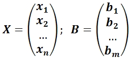
- Systems m linear equations with n unknown.
Solving a system of linear equations Is such a set of numbers ( x 1, x 2, ..., x n), when substituted into each of the equations of the system, the correct equality is obtained.
where a ij, i = 1, ..., m; j = 1,…, n- system coefficients;
b i, i = 1, ..., m- free members;
x j, j = 1, ..., n- unknown.
The above system can be written in matrix form: A X = B,
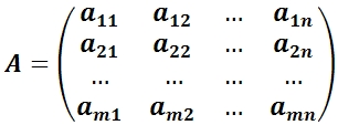
where ( A|B) Is the main matrix of the system;
A- extended system matrix;
X- column of unknowns;
B- column of free members.
If the matrix B is not a null matrix ∅, then this system of linear equations is called inhomogeneous.
If the matrix B= ∅, then this system of linear equations is called homogeneous. A homogeneous system always has a zero (trivial) solution: x 1 = x 2 =…, x n = 0.
Joint system of linear equations Is a system of linear equations that has a solution.
Inconsistent system of linear equations Is a system of linear equations that has no solution.
A definite system of linear equations Is a system of linear equations that has a unique solution.
Indefinite system of linear equations Is a system of linear equations that has an infinite set of solutions. - Systems of n linear equations with n unknowns
If the number of unknowns is equal to the number of equations, then the matrix is square. The determinant of a matrix is called the main determinant of a system of linear equations and is denoted by the symbol Δ.
Cramer's method to solve systems n linear equations with n unknown.
Cramer's rule.
If the main determinant of the system of linear equations is not is zero, then the system is consistent and defined, and the only solution is calculated by Cramer's formulas:
where Δ i - determinants obtained from the main determinant of the system Δ by replacing i th column per free member column. ... - Systems of m linear equations with n unknowns
Kronecker-Capelli theorem.
For a given system of linear equations to be consistent, it is necessary and sufficient that the rank of the matrix of the system be equal to the rank of the extended matrix of the system, rang (Α) = rang (Α | B).
If rang (Α) ≠ rang (Α | B), then the system certainly has no solutions.
If rang (Α) = rang (Α | B), then two cases are possible:
1) rang (Α) = n(to the number of unknowns) - the solution is unique and can be obtained by Cramer's formulas;
2) rang (Α)< n - there are infinitely many solutions. - Gauss method for solving systems of linear equations
Let's compose an expanded matrix ( A|B) of a given system of coefficients at unknown and right-hand sides.
The Gauss method or the method of eliminating unknowns consists in reducing the extended matrix ( A|B) with the help of elementary transformations over its rows to the diagonal form (to the upper triangular form). Returning to the system of equations, all unknowns are determined.
TO elementary transformations above the lines include the following:
1) swapping two lines;
2) multiplying a string by a number other than 0;
3) adding to the string another string multiplied by an arbitrary number;
4) throwing out the null string.
The expanded matrix, reduced to a diagonal form, corresponds linear system, which is equivalent to the given one, the solution of which is not difficult. ... - System of homogeneous linear equations.
A homogeneous system looks like:
it matches matrix equation A X = 0.
1) A homogeneous system is always compatible, since r (A) = r (A | B), there is always a zero solution (0, 0,…, 0).
2) For a homogeneous system to have a nonzero solution, it is necessary and sufficient that r = r (A)< n , which is equivalent to Δ = 0.
3) If r< n , then deliberately Δ = 0, then free unknowns arise c 1, c 2, ..., c n-r, the system has nontrivial solutions, and there are infinitely many of them.
4) General solution X at r< n can be written in matrix form as follows:
X = c 1 X 1 + c 2 X 2 +… + c n-r X n-r,
where are the solutions X 1, X 2, ..., X n-r form a fundamental system of decisions.
5) The fundamental system of solutions can be obtained from the general solution of a homogeneous system: ,
,
if the parameter values are sequentially assumed to be (1, 0,…, 0), (0, 1,…, 0),…, (0, 0,…, 1).
Decomposition of the general solution with respect to fundamental system decisions Is a record of a general solution in the form of a linear combination of solutions belonging to the fundamental system.
Theorem... In order for the system of linear homogeneous equations has a nonzero solution, it is necessary and sufficient that Δ ≠ 0.
So, if the determinant Δ ≠ 0, then the system has a unique solution.
If Δ ≠ 0, then the system of linear homogeneous equations has an infinite set of solutions.
Theorem... For a homogeneous system to have a nonzero solution, it is necessary and sufficient that r (A)< n .
Proof:
1) r can't be more n(the rank of the matrix does not exceed the number of columns or rows);
2) r< n since if r = n, then the main determinant of the system is Δ ≠ 0, and, according to Cramer's formulas, there is a unique trivial solution x 1 = x 2 =… = x n = 0, which contradicts the condition. Means, r (A)< n .
Consequence... In order for a homogeneous system n linear equations with n unknowns has a nonzero solution, it is necessary and sufficient that Δ = 0.