Correlation and regression. Correlation-regression analysis in Excel: execution instruction

Service purpose... Using the service online, you can find:

equation parameters linear regression y = a + bx, linear coefficient correlations with checking its significance;
tightness of communication using indicators of correlation and determination, OLS-assessment, static reliability regression modeling using Fisher's F-test and Student's t-test, confidence interval forecast for significance level α

Pairwise regression equation refers to first order regression equation... If the econometric model contains only one explanatory variable, then it is called pair regression. Second order regression equation and third order regression equation refer to nonlinear regression equations.

An example. Select the dependent (explained) and explanatory variable to build a paired regression model. Give . Determine the theoretical pairwise regression equation. Evaluate the adequacy of the constructed model (interpret the R-square, t-statistics, F-statistics).
Solution will be carried out on the basis of econometric modeling process.
1st stage (staged) - determination of the ultimate goals of modeling, a set of factors and indicators participating in the model, and their role.
Model specification - definition of the research goal and selection of economic variables of the model.
Situational (practical) task. For 10 enterprises in the region, the dependence of output per employee y (thousand rubles) on specific gravity highly skilled workers in the total number of workers x (in%).
2nd stage (a priori) - a pre-model analysis of the economic essence of the phenomenon under study, the formation and formalization of a priori information and initial assumptions, in particular related to the nature and genesis of the initial statistical data and random residual components in the form of a number of hypotheses.
Already at this stage, we can talk about an explicit dependence of the level of qualifications of the worker and his production, because the more experienced the worker, the higher his productivity. But how is this dependence to be assessed?
Pairwise regression is a regression between two variables - y and x, i.e. a model of the form:

Where y is the dependent variable (performance indicator); x is an independent, or explanatory, variable (sign factor). The “^” sign means that there is no strict functional dependence between the variables x and y, therefore, in almost every individual case, the value of y is the sum of two terms:

Where y is the actual value of the effective attribute; y x - the theoretical value of the effective indicator, found on the basis of the regression equation; ε - random value, characterizing the deviation of the real value of the effective indicator from the theoretical, found by the regression equation.
Let us graphically show the regression relationship between the output per worker and the share of highly skilled workers.

3rd stage (parameterization) - the actual modeling, i.e. choice general view model, including the composition and form of the relationships between variables included in it. The choice of the type of functional dependence in the regression equation is called parameterization of the model. We choose pair regression equation, i.e. only one factor will affect the final result y.
4th stage (informational) - collection of the necessary statistical information, i.e. registration of the values of the factors and indicators involved in the model. The sample consists of 10 companies in the industry.
5th stage (model identification) - estimation of unknown parameters of the model according to the available statistical data.
To determine the parameters of the model, we use OLS - method least squares ... The system of normal equations will look like this:
a n + b∑x = ∑y
a∑x + b∑x 2 = ∑y x
To calculate the parameters of the regression, let's build a calculation table (Table 1).

x	y	x 2	y 2	x y
10	6	100	36	60
12	6	144	36	72
15	7	225	49	105
17	7	289	49	119
18	7	324	49	126
19	8	361	64	152
19	8	361	64	152
20	9	400	81	180
20	9	400	81	180
21	10	441	100	210
171	77	3045	609	1356

We take the data from Table 1 (the last row), as a result we have:
10a + 171 b = 77
171 a + 3045 b = 1356
We solve this SLAE by the Cramer method or by the inverse matrix method.
We get empirical regression coefficients: b = 0.3251, a = 2.1414
The empirical regression equation is:
y = 0.3251 x + 2.1414
6th stage (model verification) - comparison of real and model data, checking the adequacy of the model, assessing the accuracy of the model data.
The analysis is carried out using

MS Excel allows you to do most of the work very quickly when constructing a linear regression equation. It is important to understand how to interpret the results obtained. To build a regression model, select the Service \ Data Analysis \ Regression item (in Excel 2007 this mode is located in the Data / Data Analysis / Regression section). Then copy the obtained results into the block for analysis.

Linear regression allows us to describe a straight line that best matches a series of ordered pairs (x, y). Equation for a straight line known as linear equation, presented below:

ŷ is the expected value of y for a given value of x,

x is an independent variable,

a - segment on the y-axis for a straight line,

b - slope of a straight line.

The figure below shows this concept graphically:

The picture above shows the line described by the equation ŷ = 2 + 0.5x. The segment on the y-axis is the point of intersection of the line with the y-axis; in our case a = 2. The slope of the line, b, the ratio of the rise of the line to the length of the line, has a value of 0.5. A positive slope means the line is going up from left to right. If b = 0, the line is horizontal, which means that there is no relationship between the dependent and independent variables. In other words, changing the x value does not affect the y value.

Often confused with ŷ and y. The graph shows 6 ordered pairs of points and a line according to this equation

This figure shows the point corresponding to the ordered pair x = 2 and y = 4. Note that the expected value of y according to the line at NS= 2 is ŷ. We can confirm this with the following equation:

ŷ = 2 + 0.5x = 2 +0.5 (2) = 3.

The y-value is the actual point, and the-value is the expected y-value using a linear equation at a given x-value.

The next step is to determine the linear equation that most closely matches the set of ordered pairs, we talked about this in the previous article, where we determined the form of the equation by.

Using Excel to Define Linear Regression

In order to use the regression analysis tool built into Excel, you must activate the add-in Analysis package... You can find it by clicking on the tab File -> Options(2007+), in the dialog box that appears ParametersExcel go to the tab Add-ons. In field Control choose Add-onsExcel and click Go. In the window that appears, put a tick opposite Analysis package, we press OK.

In the tab Data in Group Analysis a new button will appear Data analysis.

To demonstrate how the add-in works, let's use the data where a guy and a girl share a table in the bathroom. Enter the data for our bathtub example in columns A and B of the blank slate.

Go to the tab Data, in Group Analysis click Data analysis. In the window that appears Data analysis choose Regression as shown and click OK.

Set the required regression parameters in the window Regression, as it shown on the picture:

Click OK. The figure below shows the results obtained:

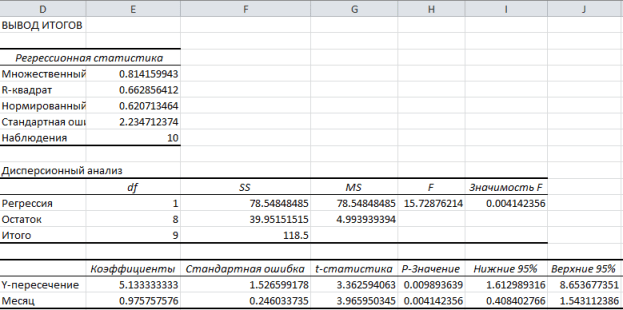
These results are consistent with those we obtained through our own calculations in.

In previous posts, the analysis often focused on a single numerical variable, such as mutual fund returns, Web page load times, or soft drink consumption. In this and the following notes, we will consider methods for predicting the values of a numeric variable depending on the values of one or more other numeric variables.

The material will be illustrated with a cross-cutting example. Forecasting the volume of sales in a clothing store. Sunflowers chain of discount clothing stores has been constantly expanding for 25 years. However, the company currently does not have a systematic approach to selecting new outlets. The location where the company intends to open a new store is determined on the basis of subjective considerations. The selection criteria are favorable rental conditions or the manager's idea of the ideal location of the store. Imagine that you are the head of the special projects and planning department. You have been tasked with developing a strategic plan for new store openings. This plan should include a forecast for the annual sales of newly opened stores. You believe that selling space is directly related to the amount of revenue, and you want to take this fact into account in your decision-making process. How do you develop a statistical model that predicts annual sales based on new store size?

Typically, to predict the values of a variable, one uses regression analysis... Its goal is to develop a statistical model that predicts the values of the dependent variable, or response, from the values of at least one independent or explanatory variable. In this post, we'll look at simple linear regression, a statistical technique that predicts the values of the dependent variable. Y by the values of the independent variable X... The following notes will describe the model multiple regression, designed to predict the values of the independent variable Y by the values of several dependent variables ( X 1, X 2, ..., X k).

Download a note in format or, examples in format

Types of regression models

where ρ 1 - autocorrelation coefficient; if ρ 1 = 0 (no autocorrelation), D≈ 2; if ρ 1 ≈ 1 (positive autocorrelation), D≈ 0; if ρ 1 = -1 (negative autocorrelation), D ≈ 4.

In practice, the application of the Durbin-Watson test is based on a comparison of the value D with critical theoretical values d L and d U for a given number of observations n, the number of independent variables of the model k(for simple linear regression k= 1) and significance level α. If D< d L , the independence hypothesis random deviations rejected (hence positive autocorrelation is present); if D> d U, the hypothesis is not rejected (that is, there is no autocorrelation); if d L< D < d U , there is no sufficient basis for making a decision. When the calculated value D exceeds 2, then with d L and d U not the coefficient itself is compared D, and expression (4 - D).

To calculate the Durbin-Watson statistics in Excel, we turn to the bottom table in Fig. fourteen Withdrawing the remainder... The numerator in expression (10) is calculated using the function = SUMKVRAZN (array1; array2), and the denominator = SUMKV (array) (Fig. 16).

Rice. 16. Formulas for calculating the Durbin-Watson statistics

In our example D= 0.883. The main question is - what value of the Durbin-Watson statistic should be considered small enough to conclude that there is a positive autocorrelation? It is necessary to correlate the D value with the critical values ( d L and d U) depending on the number of observations n and significance level α (Fig. 17).

Rice. 17. Critical values of the Durbin-Watson statistics (fragment of the table)

Thus, in the problem of the volume of sales in a store that delivers goods to your home, there is one independent variable ( k= 1), 15 observations ( n= 15) and significance level α = 0.05. Consequently, d L= 1.08 and dU= 1.36. Because the D = 0,883 < d L= 1.08, there is a positive autocorrelation between the residuals, the least squares method cannot be used.

Testing hypotheses about slope and correlation coefficient

The above regression was used solely for forecasting. To determine regression coefficients and predict the value of a variable Y at given value variable X the least squares method was used. In addition, we looked at the root-mean-square error of the estimate and the coefficient of mixed correlation. If the analysis of residuals confirms that the conditions of applicability of the least squares method are not violated, and the simple linear regression model is adequate, based on the sample data, it can be argued that between the variables in the general population there is a linear relationship.

Applicationt - the criterion for the slope. By checking whether the slope of the population β 1 is equal to zero, it is possible to determine whether there is a statistically significant relationship between the variables X and Y... If this hypothesis is rejected, it can be argued that between the variables X and Y there is a linear relationship. The null and alternative hypotheses are formulated as follows: H 0: β 1 = 0 (there is no linear dependence), H1: β 1 ≠ 0 (there is a linear dependence). By definition t-statistics is equal to the difference between the sample slope and the hypothetical slope of the population divided by the mean square error of the slope estimate:

(11) t = (b 1 – β 1 ) / S b 1

where b 1 Is the slope of the regression line based on sample data, β1 is the hypothetical slope of the straight line of the general population, , and the test statistics t It has t-distribution with n - 2 degrees of freedom.

Let's check if there is a statistically significant relationship between store size and annual sales at α = 0.05. t-criterion is displayed along with other parameters when using Analysis package(option Regression). The complete results of the Analysis Pack are shown in Fig. 4, a fragment related to t-statistics is shown in Fig. 18.

Rice. 18. Application results t

Since the number of stores n= 14 (see Fig. 3), critical importance t-statistics at a significance level of α = 0.05 can be found by the formula: t L= STUDENT.OBR (0.025; 12) = –2.1788, where 0.025 is half the significance level, and 12 = n – 2; t U= STUDENT.OBR (0.975; 12) = +2.1788.

Because the t-statistics = 10.64> t U= 2.1788 (Fig. 19), null hypothesis H 0 deviates. On the other side, R-value for NS= 10.6411, calculated by the formula = 1-STUDENT.DIST (D3; 12; TRUE), is approximately equal to zero, therefore the hypothesis H 0 deviates again. The fact that R-value almost equal to zero means that if there were no real linear relationship between store size and annual sales, it would be almost impossible to detect it using linear regression. Consequently, there is a statistically significant linear relationship between the average annual sales in stores and their size.

Rice. 19. Testing the hypothesis about the slope of the general population at a significance level of 0.05 and 12 degrees of freedom

ApplicationF - the criterion for the slope. An alternative approach to testing slope hypotheses of simple linear regression is to use F-criterion. Recall that F-criterion is used to test the relationship between two variances (see details). When testing the slope hypothesis, the measure of random errors is the error variance (the sum of the squared errors divided by the number of degrees of freedom), therefore F-criterion uses the ratio of variance explained by the regression (i.e., the values SSR divided by the number of independent variables k), to the variance of errors ( MSE = S YX 2 ).

By definition F-Statistics is equal to the mean square of the deviation due to regression (MSR) divided by the variance of the error (MSE): F = MSR/ MSE, where MSR =SSR / k, MSE =SSE/(n- k - 1), k- the number of independent variables in the regression model. Test statistics F It has F-distribution with k and n- k - 1 degrees of freedom.

For a given significance level α, the decision rule is formulated as follows: if F> FU, the null hypothesis is rejected; otherwise, it is not rejected. The results, presented in the form of a summary table of analysis of variance, are shown in Fig. twenty.

Rice. 20. ANOVA table to test the hypothesis about statistical significance regression coefficient

Likewise t-criterion F-criterion is displayed in the table when used Analysis package(option Regression). Completely results of work Analysis package are shown in Fig. 4, a fragment related to F-statistics - in Fig. 21.

Rice. 21. Application results F-criteria obtained using the Excel Analysis Package

The F statistic is 113.23 and R-value close to zero (cell SignificanceF). If the significance level α is 0.05, determine the critical value F-distributions with one and 12 degrees of freedom can be given by the formula F U= F. OBR (1-0.05; 1; 12) = 4.7472 (Fig. 22). Because the F = 113,23 > F U= 4.7472, and R-value close to 0< 0,05, нулевая гипотеза H 0 deviates, i.e. store size is closely related to its annual sales.

Rice. 22. Testing the hypothesis about the slope of the general population at a significance level of 0.05, with one and 12 degrees of freedom

Confidence interval containing the slope β 1. To test the hypothesis about the existence of a linear relationship between the variables, you can build a confidence interval containing the slope β 1 and make sure that the hypothetical value β 1 = 0 belongs to this interval. The center of the confidence interval containing the slope β 1 is the sample slope b 1 , and its boundaries are the quantities b 1 ±t n –2 S b 1

As shown in fig. 18, b 1 = +1,670, n = 14, S b 1 = 0,157. t 12 = STUDENT.OBR (0.975; 12) = 2.1788. Consequently, b 1 ±t n –2 S b 1 = +1.670 ± 2.1788 * 0.157 = +1.670 ± 0.342, or + 1.328 ≤ β 1 ≤ +2.012. Thus, the slope of the general population with a probability of 0.95 lies in the range from +1.328 to +2.012 (ie, from $ 1,328,000 to $ 2,012,000). Since these values are greater than zero, there is a statistically significant linear relationship between annual sales and store area. If the confidence interval contained zero, there would be no dependency between the variables. In addition, the confidence interval means that each increase in store area by 1,000 sq. M. feet results in an increase in average sales of $ 1,328,000 to $ 2,012,000.

Usaget -criterion for the correlation coefficient. correlation coefficient was introduced r, which is a measure of the relationship between two numeric variables. It can be used to determine whether there is a statistically significant relationship between two variables. Let us denote the correlation coefficient between the general populations of both variables by the symbol ρ. The null and alternative hypotheses are formulated as follows: H 0: ρ = 0 (no correlation), H 1: ρ ≠ 0 (there is a correlation). Checking for the existence of a correlation:

where r = + , if b 1 > 0, r = – , if b 1 < 0. Тестовая статистика t It has t-distribution with n - 2 degrees of freedom.

In the problem about the chain of stores Sunflowers r 2= 0.904, and b 1- +1.670 (see fig. 4). Because the b 1> 0, the correlation coefficient between annual sales and store size is r= + √0.904 = +0.951. Check the null hypothesis that there is no correlation between these variables using t-statistics:

At a significance level of α = 0.05, the null hypothesis should be rejected because t= 10.64> 2.1788. Thus, it can be argued that there is a statistically significant relationship between annual sales and store size.

Confidence intervals and criteria for testing hypotheses are used interchangeably when discussing conclusions about population slope. However, calculating the confidence interval containing the correlation coefficient turns out to be more difficult, since the form of the sample distribution of the statistic r depends on the true correlation coefficient.

Estimation of mathematical expectation and prediction of individual values

This section discusses methods for evaluating the expected response Y and predictions of individual values Y at the given values of the variable X.

Building a confidence interval. In example 2 (see section above Least square method) regression equation made it possible to predict the value of a variable Y X... In the problem of choosing a place for point of sale average annual sales for a 4,000 sqm store ft was equal to $ 7.644 million. However, this estimate of the mathematical expectation of the general population is pointwise. to assess the mathematical expectation of the general population, the concept of a confidence interval was proposed. Similarly, we can introduce the concept confidence interval for the expected response for a given value of the variable X:

where , = b 0 + b 1 X i- the predicted value is variable Y at X = X i, S YX- root-mean-square error, n- sample size, Xi- the set value of the variable X, µ Y|X = Xi – expected value variable Y at NS = X i, SSX =

Analysis of formula (13) shows that the width of the confidence interval depends on several factors. At a given level of significance, an increase in the amplitude of oscillations around the regression line, measured using the root mean square error, leads to an increase in the width of the interval. On the other hand, as expected, an increase in the sample size is accompanied by a narrowing of the interval. In addition, the width of the interval changes depending on the values Xi... If the value of the variable Y predicted for quantities X close to the mean , the confidence interval turns out to be narrower than when predicting the response for values far from the mean.

Suppose that when choosing a location for a store, we want to plot a 95% confidence interval for the average annual sales of all stores with an area of 4,000 square meters. feet:

Consequently, the average annual sales in all stores with an area of 4,000 square meters. feet, with a 95% probability lies in the range from 6.971 to 8.317 million dollars.

Calculating the confidence interval for the predicted value. In addition to the confidence interval for the mathematical expectation of the response at a given value of the variable X, it is often necessary to know the confidence interval for the predicted value. Despite the fact that the formula for calculating this confidence interval is very similar to formula (13), this interval contains the predicted value, not the parameter estimate. Predicted response interval YX = Xi at a specific value of the variable Xi determined by the formula:

Suppose that when choosing a location for a store, we want to plot a 95% confidence interval for the predicted annual sales of a store with an area of 4000 sq. feet:

Therefore, the predicted annual sales volume for a store with an area of 4000 sq. ft, with a 95% probability lies in the range from 5.433 to 9.854 million dollars. As you can see, the confidence interval for the predicted value of the response is much wider than the confidence interval for its mathematical expectation. This is due to the fact that the variability in predicting individual values is much greater than when assessing the mathematical expectation.

Pitfalls and Ethical Issues with Regression

Difficulties with regression analysis:

Ignoring the conditions of applicability of the least squares method.
Erroneous assessment of the conditions of applicability of the least squares method.
Wrong choice of alternative methods when the conditions of applicability of the least squares method are violated.
Application of regression analysis without deep knowledge of the subject of research.
Extrapolation of the regression beyond the range of the explanatory variable.
Confusion between statistical and causal relationships.

Widespread spread of spreadsheets and software for statistical calculations eliminated the computational problems that prevented the application of regression analysis. However, this led to the fact that the regression analysis began to be used by users who do not have sufficient qualifications and knowledge. How do users know about alternative methods, if many of them have no idea at all about the conditions for the applicability of the least squares method and do not know how to verify their implementation?

The researcher should not get carried away with grinding numbers - calculating shift, slope, and mixed correlation coefficient. He needs deeper knowledge. Let us illustrate this classic example taken from textbooks. Anscombe showed that all four datasets shown in Fig. 23 have the same regression parameters (Fig. 24).

Rice. 23. Four sets of artificial data

Rice. 24. Regression analysis of four artificial datasets; done with Analysis package(click on the picture to enlarge the picture)

So, from the point of view of regression analysis, all these datasets are completely identical. If the analysis were over, we would have lost a lot. useful information... This is evidenced by the scatter plots (Figure 25) and residual plots (Figure 26) plotted for these datasets.

Rice. 25. Scatter plots for four datasets

Scatter plots and residual plots show that these data differ from each other. The only set distributed along a straight line is set A. The plot of the residuals calculated from set A has no regularity. The same cannot be said for Sets B, C, and D. The scatter plot plotted for Set B demonstrates a pronounced quadratic model. This conclusion is confirmed by the plot of the residuals, which has a parabolic shape. The scatter plot and the residual plot show that dataset B contains an outlier. In this situation, it is necessary to exclude the outlier from the dataset and repeat the analysis. A technique for detecting and eliminating outliers from observations is called impact analysis. After eliminating the outlier, the result of reevaluating the model may be completely different. A scatter plot from dataset D illustrates the unusual situation in which the empirical model is highly dependent on an individual response ( X 8 = 19, Y 8 = 12.5). Such regression models need to be computed with particular care. So, the scatter and residual plots are extremely necessary tool regression analysis and should be an integral part of it. Without them, regression analysis is untrustworthy.

Rice. 26. Plots of residuals for four datasets

How to avoid pitfalls in regression analysis:

Analysis of the possible relationship between variables X and Y always start by plotting a scatter chart.
Check the applicability conditions before interpreting the results of the regression analysis.
Plot the residuals versus the independent variable. This will allow you to determine how the empirical model is consistent with the observation results, and to detect a violation of the constancy of variance.
Use histograms, stem and leaf plots, box plots, and normal distribution plots to test the normal error assumption.
If the conditions of applicability of the least squares method are not met, use alternative methods(for example, quadratic or multiple regression models).
If the conditions for the applicability of the least squares method are met, it is necessary to test the hypothesis about the statistical significance of the regression coefficients and build confidence intervals containing the mathematical expectation and the predicted response value.
Avoid predicting values of the dependent variable outside the range of the independent variable.
Keep in mind that statistical relationships are not always causal. Remember that correlation between variables does not mean there is a causal relationship between them.

Summary. As shown in the block diagram (Fig. 27), the note describes the simple linear regression model, the conditions for its applicability and how to check these conditions. Considered t-criterion for checking the statistical significance of the slope of the regression. A regression model was used to predict the values of the dependent variable. An example is considered related to the choice of a location for a retail outlet, in which the dependence of the annual sales volume on the area of the store is investigated. The information obtained allows you to more accurately choose the location for the store and predict its annual sales. In the following notes, we will continue our discussion of regression analysis and also look at multiple regression models.

Rice. 27. Block diagram of the note

Used materials of the book Levin and other Statistics for managers. - M .: Williams, 2004 .-- p. 792-872

If the dependent variable is categorical, then logistic regression should be applied.

What is regression?

Consider two continuous variables x = (x 1, x 2, .., x n), y = (y 1, y 2, ..., y n).

Let's place the points on a 2D scatter plot and say we have linear relationship if the data is fitted with a straight line.

If we believe that y depends on x, and changes in y are caused precisely by changes in x, we can determine the regression line (regression y on the x), which best describes the straightforward relationship between the two variables.

The statistical use of the word "regression" comes from a phenomenon known as regression to the mean, attributed to Sir Francis Galton (1889).

He showed that although tall fathers tend to have tall sons, the average height of sons is shorter than that of their tall fathers. The average height of sons "regressed" and "reversed" to the average height of all fathers in the population. Thus, on average, tall fathers have lower (but still tall) sons, and lower fathers have higher (but still rather short) sons.

Regression line

A mathematical equation that estimates a simple (paired) linear regression line:

x called the independent variable or predictor.

Y- dependent variable or response variable. This is the value we expect for y(on average) if we know the value x, i.e. this "predicted value y»

a- free member (intersection) of the line of evaluation; this value Y, when x = 0(Fig. 1).
b - slope or the gradient of the evaluated line; it represents the amount by which Y increases on average if we increase x by one unit.
a and b are called the regression coefficients of the estimated line, although this term is often used only for b.

Paired linear regression can be extended to include more than one independent variable; in this case it is known as multiple regression.

Fig. 1. Linear regression line showing the intersection of a and the slope of b (the amount of Y increases as x increases by one unit)

Least square method

We perform regression analysis using a sample of observations where a and b- sample estimates of the true (general) parameters, α and β, which determine the line of linear regression in the population (general population).

Most simple method determination of coefficients a and b is an least square method(OLS).

The fit is estimated by considering the residuals (the vertical distance of each point from the line, for example, residual = observed y- predicted y, Rice. 2).

The best fit line is chosen so that the sum of the squares of the residuals is minimal.

Rice. 2. Linear regression line with residuals depicted (vertical dashed lines) for each point.

Linear Regression Assumptions

So, for each observed value, the residual is equal to the difference and the corresponding predicted value. Each residual can be positive or negative.

You can use the residuals to test the following assumptions underlying linear regression:

The balances are normally distributed with a zero mean;

If the assumptions of linearity, normality and / or constant variance are questionable, we can transform or and calculate a new regression line for which these assumptions are satisfied (for example, use a log transformation, etc.).

Abnormal values (outliers) and influence points

An "influential" observation, if omitted, changes one or more estimates of model parameters (ie, slope or intercept).

An outlier (an observation that contradicts most of the values in a dataset) can be an “influential” observation and can be well detected visually when viewed from a 2D scatter plot or a residual plot.

For both outliers and "influential" observations (points), models are used, both with and without them, and they pay attention to the change in the estimate (regression coefficients).

When performing analysis, do not automatically discard outliers or influence points, as simple ignoring can affect the results obtained. Always investigate and analyze the causes of these outliers.

Linear regression hypothesis

When constructing a linear regression, the null hypothesis is tested that the general slope of the regression line β is zero.

If the slope of the line is zero, there is no linear relationship between and: the change does not affect

To test the null hypothesis that the true slope is zero, you can use the following algorithm:

Calculate a test statistic equal to the ratio that obeys a distribution with degrees of freedom, where the standard error of the coefficient is

- estimation of the variance of the residuals.

Usually, if the level of significance achieved is the null hypothesis is rejected.

where is the percentage point of the distribution with degrees of freedom that gives the probability of a two-sided test

This is the interval that contains the general slope with a 95% probability.

For large samples, say we can approximate with a value of 1.96 (that is, the criterion statistics will tend to normal distribution)

Evaluation of the quality of linear regression: coefficient of determination R 2

Because of the linear relationship, and we expect it to change as it changes , and we call this variation that is caused or explained by regression. The residual variation should be as small as possible.

If this is the case, then most of the variation will be due to regression, and the points will lie close to the regression line, i.e. the line matches the data well.

Share total variance, which is explained by the regression is called coefficient of determination, usually expressed in terms of percentage and denote R 2(in paired linear regression, this is the value r 2, the square of the correlation coefficient), allows you to subjectively assess the quality of the regression equation.

The difference is the percentage of variance that cannot be explained by the regression.

There is no formal test to evaluate, we have to rely on subjective judgment to determine the quality of the regression line fit.

Applying a regression line to forecast

You can use a regression line to predict a value from a value within the observed range (never extrapolate outside these limits).

We predict the mean for observables that have a particular value by plugging that value into the regression line equation.

So, if we predict how We use this predicted value and its standard error to estimate the confidence interval for the true mean in the population.

Repeating this procedure for different values allows you to build confidence limits for this line. This is the band or area that contains the true line, for example, with a 95% confidence level.

Simple regression designs

Simple regression designs contain one continuous predictor. If there are 3 cases with P predictor values, for example, 7, 4, and 9, and the design includes a first-order effect P, then the design matrix X will have the form

and the regression equation using P for X1 looks like

Y = b0 + b1 P

If a simple regression design contains a higher order effect on P, such as a quadratic effect, then the values in column X1 in the design matrix will be raised to the second power:

and the equation takes the form

Y = b0 + b1 P2

Sigma-restricted and overparameterized coding methods do not apply to simple regression designs and other designs containing only continuous predictors (since categorical predictors simply do not exist). Regardless of the coding method chosen, the values of the continuous variables are increased to the appropriate degree and used as the values for the X variables. In this case, no recoding is performed. In addition, when describing regression designs, you can omit consideration of the design matrix X, and work only with the regression equation.

Example: Simple Regression Analysis

This example uses the data presented in the table:

Rice. 3. Table of initial data.

Data compiled from a comparison of the 1960 and 1970 census in a randomly selected 30 districts. District names are represented as observation names. Information regarding each variable is presented below:

Rice. 4. Table of variable specifications.

Research task

For this example, the correlation between the poverty rate and the degree will be analyzed, which predicts the percentage of families that are below the poverty line. Therefore, we will treat variable 3 (Pt_Poor) as a dependent variable.

It can be hypothesized that population change and the percentage of families below the poverty line are related. It seems reasonable to expect that poverty leads to population outflow, hence there will be a negative correlation between the percentage of people below the poverty line and population change. Therefore, we will treat variable 1 (Pop_Chng) as a predictor variable.

Viewing Results

Regression coefficients

Rice. 5. Regression coefficients Pt_Poor on Pop_Chng.

At the intersection of the Pop_Chng row and the Param. the non-standardized coefficient for the Pt_Poor regression on Pop_Chng is -0.40374. This means that for every unit decrease in population, there is a 40374 increase in the poverty rate. The upper and lower (default) 95% confidence limits for this non-standardized coefficient do not include zero, so the regression coefficient is significant at the p level<.05 . Обратите внимание на не стандартизованный коэффициент, который также является коэффициентом корреляции Пирсона для простых регрессионных планов, равен -.65, который означает, что для каждого уменьшения стандартного отклонения численности населения происходит увеличение стандартного отклонения уровня бедности на.65.

Distribution of variables

Correlation coefficients can become significantly overestimated or underestimated if there are large outliers in the data. Let us examine the distribution of the dependent variable Pt_Poor by district. To do this, let's build a histogram of the Pt_Poor variable.

Rice. 6. Histogram of the Pt_Poor variable.

As you can see, the distribution of this variable differs markedly from the normal distribution. However, although even the two counties (the two right-hand columns) have a higher percentage of households below the poverty line than expected from the normal distribution, they appear to be "within the range."

Rice. 7. Histogram of the Pt_Poor variable.

This judgment is somewhat subjective. As a rule of thumb, outliers must be accounted for if the observation (or observations) do not fall within the interval (mean ± 3 times the standard deviation). In this case, it is worth repeating the analysis with and without outliers to ensure that they do not have a significant effect on the correlation between members of the population.

Scatter plot

If one of the hypotheses is a priori about the relationship between the given variables, then it is useful to check it on the graph of the corresponding scatterplot.

Rice. 8. Scatter diagram.

The scatter plot shows a clear negative correlation (-.65) between the two variables. It also shows the 95% confidence interval for the regression line, that is, with a 95% probability the regression line falls between the two dashed curves.

Significance criteria

Rice. 9. Table containing criteria for significance.

The criterion for the Pop_Chng regression coefficient confirms that Pop_Chng is strongly related to Pt_Poor, p<.001 .

Outcome

This example showed how to analyze a simple regression design. An interpretation of the non-standardized and standardized regression coefficients was also presented. The importance of studying the distribution of responses of the dependent variable is discussed, and a technique for determining the direction and strength of the relationship between the predictor and the dependent variable is demonstrated.