Making a table in excel. How rows and columns are highlighted

Excel is a multifunctional application, the functionality of which clearly exceeds the capabilities of any other. Economists, accountants, etc. cannot do without this application. specialists. Excel allows you to draw all kinds of graphs, tables, etc., which greatly simplifies life.

However, despite the sheer number of features, tables are still the most basic feature most used by users. It is precisely because of the need to draw a beautiful table, say, for a presentation or for work, that many download Excel and, of course, do it right. After all, this program is ideally tailored to perform such actions, and tables can have all kinds of shapes and sizes, and, moreover, it is very simple! But let's talk about everything in order. So, next we will talk about how to make tables in excel.

How to draw a table in Excel

How to work with a table

Now you can correct the table itself, change/add data, delete/add rows and columns, thereby expanding the boundaries of the table, etc. So, for example, if you hover over the bottom corner of the table and drag it, it will start to grow, and you can also reduce it in the same way.

The table can be made a little larger. To do this, select any row or column and right-click on it. A menu will pop up in which you need to select the “Insert” item, and then any of the listed lines, for example, “Table columns on the left”. In this way, your plate can be overgrown with new elements. Also, according to the table, you can. I hope that the question of how to work with tables in excel has become more understandable for you!

Of course, it will not be possible to consider all the nuances, there are too many of them. But the most basic, so to speak, the basics, you now know, and then it's up to the small - draw the table yourself!

Video to help

To simplify the management of logically related data, EXCEL 2007 introduces a new table format. Using tables in EXCEL 2007 format reduces the possibility of entering incorrect data, simplifies the insertion and deletion of rows and columns, and simplifies table formatting.

Source table

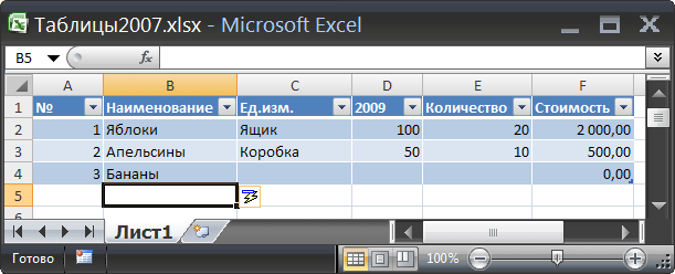
Let there be a regular table (a range of cells) consisting of 6 columns.

In column № (position number), starting from the second row of the table, there is a formula =A2+1 that allows you to perform automatic . To speed up the entry of values in a column Unit.(unit) using created .

In column Price introduced a formula for calculating the cost of goods (price*quantity) =E3*D3 . Numeric values in a column are formatted to display thousands separators.

Actions with a regular table

To show the advantages of tables in the EXCEL 2007 format, we will first perform basic operations with a regular table.

First, let's add a new row to the table, i.e. Fill in line 4 of the sheet with data:

fill in the columns without formulas ( Name, Price, Quantity);
in columns Price And № use to copy the formulas into the cells below;
to work in a new line, in a column Unit. copy the format to the cell below. To do this, select a cell C3 , copy it to Clipboard and by highlighting the cell below, through the menu Home/ Clipboard/ Paste/ Paste Special/ Value Conditions insert Drop-down list(or, as in the previous step, copy the value from the cell C3 in C4 , thus copying the rule . You must then enter the Units value on a new line).

Of course, you can copy the formulas and cell formats down several lines in advance - this will speed up the filling of the table.

Now consider the same steps, but in a spreadsheet in EXCEL 2007 format.

Creating tables in EXCEL 2007 format

Select any cell of the table discussed above and select the menu item Insert/ Tables/ Table.

EXCEL will automatically detect that our table has column headings. If you uncheck Table with headers, then headings will be created for each column Column1, Column2, …

ADVICE:
Avoid headings in number formats (such as "2009") and links to them. When creating a table, they will be converted to text format. Formulas that use numeric headings as arguments may stop working.

After clicking OK:

the table will be automatically styled with interlaced highlighting;
in the header will be enabled (to disable it, select any cell in the table and press CTRL+SHIFT+L, pressing again will turn on the filter);
a special tab in the menu for working with tables will become available ( Working with tables / Constructor), the tab is active only when any table cell is selected;
the table will be assigned , which can be viewed through the table designer or through Name Manager (Formulas/ Defined Names/ Name Manager) .

ADVICE :
Before converting a table to EXCEL 2007 format, make sure that the source table is properly structured. The article outlines the basic requirements for a "correct" table structure.

Deleting tables in EXCEL 2007 format

To delete a table along with data, you need to select any heading in the table, click CTRL+ A, then key DELETE(any select any cell with data, double click CTRL+ A, then key DELETE). Another way to delete a table is to delete all rows or columns containing table cells from the sheet (you can delete rows, for example, by selecting the desired rows for the headers, right-clicking the context menu and selecting the item Delete).

To save the table data, you can convert it to a regular range. To do this, select any cell in the table (The Table Tools tab containing the Design tab will be displayed) and through the menu Working with tables / Constructor / Service / Convert to range convert it to a regular range. The table formatting will remain. If you also want to remove the formatting, clear the table style before converting to a range ( Working with tables/ Designer/ Table styles/ Clear).

Adding new lines

Now let's do the same actions with the table in EXCEL 2007 format that we did earlier with the usual range.

Let's start by filling from the column Name(first column without formulas). After entering the value, a new row will be automatically added to the table.

As you can see from the picture above, the table formatting will automatically propagate to the new line. The formulas in the columns will also be copied to the row. Price And №. In column Unit. will become available with a list of units of measurement.

To add new rows in the middle of a table, select any cell in the table above which you want to insert a new row. Right-click to call the context menu, select the menu item Insert (with an arrow), then the item Table rows above.

Removing rows

Select one or more cells in the table rows that you want to delete.
Right-click, select Delete from the context menu, and then select Table Rows. Only the table row will be deleted, not the entire sheet row.
Columns can be removed in the same way.

Table totals data

Click anywhere in the table. On the Design tab, in the Table Style Options group, select the Total Row check box.

The last row of the table will have a total row, and the leftmost cell will display the word Outcome.

In the total row, click the cell in the column for which you want to calculate the total value, and then click the drop-down arrow that appears. From the drop-down list, select the function that will be used to calculate the total.
The formulas that can be used in the totals row are not limited to formulas in the list. You can enter any formula you want in any cell in the totals row.
Once a total row has been created, adding new rows to the table is difficult because rows are no longer added automatically when new values are added (see section ). But there is nothing to worry about: the results can be disabled/enabled via the menu.

Naming Tables

When creating tables in EXCEL 2007 format, EXCEL assigns tables automatically: Table 1, Table 2 etc., but these names can be changed (via the table constructor: ) to make them more expressive.

The table name cannot be deleted (for example, via Name Manager). As long as the table exists, its name will also be determined.

Structured references (referencing fields and table values in formulas)

Now we will create a formula in which one of the columns of the table in EXCEL 2007 format is specified as arguments (we will create the formula outside the row results).

Enter in a cell H1 part of the formula: =SUM(
Select range with mouse F 2: F 4 (whole column Price No title)

But, instead of the formula =SUM(F2:F4 we will see =SUM(Table1[Cost]

This is a structured link. In this case, it's a reference to an entire column. If new rows are added to the table, then the formula =SUM(Table1[Cost]) will return the correct result given the newline value. Table 1 is the name of the table ( Working with tables/ Constructor/ Properties/ Table name).

Consider another example of summing a table column through its . In a cell H2 enter =SUM(T (the letter T is the first letter of the table name). EXCEL will prompt you to choose, starting with "T", a function or a name defined in this book (including table names).

By double-clicking on the table name, the formula will take the form =SUM(Table1. Now enter the symbol [ (open square bracket). EXCEL after entering =SUM(Table1[ will prompt you to select a specific table field. Select the field Price by double clicking on it.

into the formula =SUM(Table1[Cost enter the symbol ] (closing square bracket) and press the key ENTER. As a result, we get the sum of the column Price.

The following are other types of structured links:
Column heading link: =Table1[[#Headers];[Cost]]
Referencing a value on the same line =Table1[[#This row];[Cost]]

Copy formulas with structured references

Let there be a table with columns Price And Price with VAT. Let's assume that to the right of the table you want to calculate the total cost and the total cost with VAT.

First, calculate the total cost using the formula =SUM(Table1[Cost]). We write the formula as shown in the previous section.

Now select a cell J2 and press the key combination CTRL+R(copy the formula from the cell on the left). Unlike we get the formula =SUM(Table1[Cost]), but not =SUM(Table1[Cost with VAT]). In this case, a structured reference is like

Now let's look at a similar table and make a small one based on its data to calculate the total cost for each item of fruit.

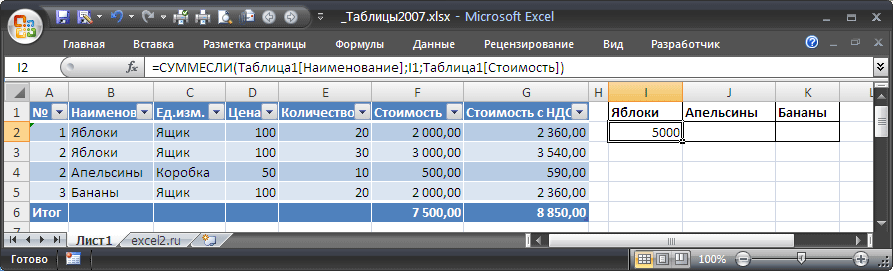
In the first row of the report (range of cells I1:K2 ) contains the names of fruits (without repetitions), and in the second line, in the cell I2 formula =SUMIF(Table1[Name],I1,Table1[Cost]) to find the total value of the fruit Apples. When copying a formula using to a cell J2 (to find the total value of the fruit oranges) the formula will become incorrect =SUMIF(Table1[Unit],J1,Table1[Cost including VAT])(see above about this), copying using a combination of keys CTRL+R solves this problem. But, if there are more names, say 20, then how to quickly copy the formula to other cells? To do this, select the desired cells (including the cell with the formula) and place the cursor in (see the figure below), then press the key combination CTRL+ENTER. The formula will be copied correctly.

Table styles

For tables created in EXCEL 2007 format ( Insert/ Tables/ Table) it is possible to use various styles to give tables a certain look, including with . Select any cell in the table, then click Constructor/ Table styles and choose the appropriate style.

Microsoft program Excel is a very powerful tool with which you can create large spreadsheets with beautiful design and an abundance of different formulas. Working with information is facilitated precisely because of the dynamics that are missing in the Word application.

This article will show you how to create a table in Excel. Thanks to step by step instructions even a “teapot” can deal with this. At first, novice users may find this difficult. But in fact, with constant work in the Excel program, you will become a professional and be able to help others.

The training plan will be simple:

first consider various methods creating tables;
Then we are engaged in design so that the information is as clear and understandable as possible.

This method is the simplest. This is done in the following way.

When you open a blank sheet, you will see a large number of identical cells.

Select any number of rows and columns.

After that, go to the "Home" tab. Click on the "Borders" icon. Then select "All".

Immediately after that, you will have the usual elementary plate.

Now you can start filling in the data.

There is another way to manually draw a table.

Click on the "Borders" icon again. But this time, select Draw Grid.

Immediately after that, you will change appearance cursor.

Make a left mouse click and drag the pointer to another position. As a result, a new grid will be drawn. The upper left corner is the initial position of the cursor. The lower right corner is the end.

The sizes can be any. The table will be created until you release your finger from the mouse button.

Auto mode

If you do not want to "work with your hands", you can always use ready-made functions. To do this, do the following.

Go to the "Insert" tab. Click on the "Tables" button and select the last item.

Pay attention to what we are prompted about hot keys. In the future, for automatic creation, you can use the combination of buttons Ctrl + T .

Immediately after that, you will see a window in which you need to specify the range of the future table.

To do this, simply select any area - the coordinates will be substituted automatically.

As soon as you release the cursor, the window will return to its original form. Click on the "OK" button.

As a result of this, a beautiful table with alternating lines will be created.

To change the name of a column, just click on it. After that, you can start editing directly in this cell or in the formula bar.

pivot table

This type of information presentation serves for its generalization and subsequent analysis. To create such an element, you need to do the following steps.

First, we create a table and fill it with some data. How to do this is described above.

Now go to the main menu "Insert". Next, we choose the option we need.

Right after that, you will have a new window.

Click on the first line (the input field must be made active). Only after that we select all the cells.

Then click on the "OK" button.

As a result of this, you will have a new sidebar where you need to configure the future table.

At this stage, you need to transfer the fields to the desired categories. The columns will be months, the rows will be the purpose of the costs, and the values will be the amount of money.

To transfer, left-click on any field and, without releasing your finger, drag the cursor to the desired location.

Only after that (the cursor icon will change appearance) can the finger be released.

As a result of these actions, you will have a new beautiful table in which everything will be calculated automatically. Most importantly, new cells will appear - “Grand Total”.

You can specify the fields that are of interest for data analysis.

Sometimes it is not possible to correctly select fields for columns and rows. And in the end, nothing worthwhile comes out. For such cases, Microsoft developers have prepared their own data analysis options.

It works very simply.

First of all, we select the information we need.

After that, select the appropriate menu item.

As a result, the program itself will analyze the contents of the cells and offer several options.

By clicking on any of the proposed options and clicking on the "OK" button, everything will be created automatically.

In the case of the example, we received the sum total costs, excluding months.

Ready-made templates in Excel 2016

For the lazy ones this program allows you to create truly "cool" tables with just one click.

When you open Excel, you have the following options to choose from:

open the latest files you have worked with before;
create a new empty workbook;
see tutorial from detailed information about the capabilities of this software;
choose some ready-made default template;
continue searching on the Internet if you don’t like any of the proposed designs;
log in under your account Microsoft.

We are interested in ready-made options. If you scroll down a bit, you will see that there are a lot of them. But these are the default templates. Imagine how many you can download them on the Internet.

Click on any option you like.

Click on the "Create" button.

As a result of this, you get ready-made version very large and complex table.

Registration

Appearance is one of the most important parameters. It is very important to focus on some elements. For example, a header, title, and so on. Everything depends on the specific case.

Consider briefly the basic manipulations with cells.

Create a header

Let's use a simple table as an example.

First, go to the "Home" tab and click on the menu item "Insert Rows to Sheet".

Select the line that appears and click on the "Merge Cells" menu item.

Next, write any title.

Changing the Height of Elements

Our header is the same size as the header. And it's not very pretty. In addition, it looks inconspicuous. In order to fix this, you need to move the cursor to the border of lines 1 and 2. After its appearance changes, left-click and drag it down.

As a result, the row height will be larger.

Text alignment

Our title is at the bottom of the cell and stuck to the header. In order to fix this, you need to use the alignment buttons. You can change the text position both vertically and horizontally.

We click on the button "In the middle" and we get the desired result.

Now the title looks much better.

Style change

Or use predefined styles. To do this, first select the line. Then, through the menu, select any of the proposed design options.

The effect will be very beautiful.

How to insert a new row or column

In order to change the number of elements in the table, you can use the "Insert" button.

You can add:

cells;
lines;
columns;
whole sheet.

Removing elements

You can destroy a cell or something else in the same way. There is a button for this.

Filling cells

If you want to highlight any column or line, you need to use the fill tool for this.

Thanks to it, you can change the color of any cells that were previously selected.

Element Format

You can do whatever you want with the table. To do this, just click on the "Format" button.

As a result of this, you will be able to:

manually or automatically change the height of the rows;
manually or automatically change the width of the columns;
hide or show cells;
rename sheet;
change label color;
protect the sheet;
block the element;
specify the cell format.

Content Format

If you click on the last of the above items, the following will appear:

With this tool, you can:

change the format of the displayed data;
specify alignment;

choose any font;

change table borders;

"play" with the fill;

set protection.

Using formulas in tables

It is thanks to the ability to use the auto-calculation functions (multiplication, addition, and so on) that Microsoft Excel has become a powerful tool.

In addition, it is recommended to read the description of all functions.

Consider the simplest operation - cell multiplication.

First, let's prepare the field for experiments.

Make active the first cell in which you want to display the result.

Enter the following command there.

=C3*D3

Now press the Enter key. After that, move the cursor over the lower right corner of this cell until its appearance changes. Then hold down the left mouse click with your finger and drag down to the last line.

As a result of autosubstitution, the formula will fall into all cells.

The values in the "Total cost" column will depend on the "Quantity" and "Cost per 1 kg" fields. That's the beauty of dynamics.

In addition, you can use ready-made functions for calculations. Let's try to calculate the sum of the last column.

First, select the values. Then click on the "Autosums" button, which is located on the "Home" tab.

As a result of this, the total sum of all numbers will appear below.

Use of graphics

Sometimes photos are used in cells instead of text. It is very easy to do this.

Select an empty element. Go to the "Insert" tab. Select the "Illustrations" section. Click on "Pictures".

Specify the file and click on the "Insert" button.

The result will not disappoint you. Looks very nice (depending on the selected pattern).

Export to Word

In order to copy data into a Word document, it is enough to do a couple of simple steps.

Select the data area.

Press the hotkeys Ctrl +C .
Open Document
Now use the buttons Ctrl + V .
The result will be as follows.

Online Services

For those who want to work in "real mode" and share information with friends or work colleagues, there is a great tool.

Using this service, you can access your documents from any device: computer, laptop, phone or tablet.

Printing methods

Printing Word documents is usually a simple task. But with tables in Excel, everything is different. The most a big problem is that "by eye" it is difficult to determine the boundaries of the print. And very often almost empty sheets appear in the printer, on which there are only 1-2 lines of the table.

Such printouts are inconvenient for perception. It is much better when all the information is on one sheet and does not go anywhere beyond the borders. In this regard, developers from Microsoft have added the function of viewing documents. Let's see how to use it.

We open the document. He looks quite normal.

Next, press the hot keys Ctrl + P . In the window that appears, we see that the information does not fit on one sheet. We have lost the column "Total cost". In addition, at the bottom we are prompted that 2 pages will be used for printing.

In the 2007 version, for this you had to click on the "View" button.

To cancel press hotkey Esc. As a result, a vertical dotted line will appear, which shows the borders of the print.

You can increase the space when printing as follows.

First of all, we reduce the margins. To do this, go to the "Page Layout" tab. Click on the "Fields" button and select the most "Narrow" option.

After that, reduce the width of the columns until the dotted line is outside the last column. How to do this was described above.

You need to reduce it within reasonable limits so that the readability of the text does not suffer.

Press Ctrl+P again. Now we see that the information is placed on one sheet.

Microsoft Product Version Differences

It should be understood that Excel 2003 has long been obsolete. There is a huge lack modern features and opportunities. In addition, the appearance various objects(graphs, diagrams, and so on) is much inferior to modern requirements.

An example of an Excel 2003 workspace.

In modern 2007, 2010, 2013, and even more so 2016 versions, everything is much “cooler”.

Many menu items are in different sections. Some of them even changed their name. For example, the “Formulas” familiar to us were called “Functions” back in 2003. And they didn't take up much space.

Now they have a whole tab dedicated to them.

Limitations and features of different versions

On the official site Microsoft you can find online help, which lists all specifications created books.

An example of the most basic parameters.

This list is quite long. Therefore, it is worth clicking on the link and familiarize yourself with the rest.

Please note that the 2003 version is not even considered, since its support has been discontinued.

But in some budget organizations this office suite is still in use today.

Conclusion

This article has reviewed various ways creating and presenting tables. Special attention was given to give a beautiful appearance. You should not overdo it in this regard, since bright colors and a variety of fonts will scare away a user who is trying to familiarize himself with the contents of the table.

Video instruction

For those who have any questions, a video is attached below, which includes additional comments on the instructions described above.

If you've never used a spreadsheet to create documents before, we recommend reading our Excel guide for dummies.

After that, you will be able to create your first spreadsheet with tables, graphs, math formulas, and formatting.

Detailed information about the basic functions and capabilities of the spreadsheet processor MS Excel. Description of the main elements of the document and instructions for working with them in our material.

Working with cells. Filling and Formatting

Before proceeding with specific actions, you need to understand the basic element of any document in Excel. An Excel file consists of one or more sheets divided into small cells.

A cell is the basic component of any Excel report, table or graph. Each cell contains one block of information. This can be a number, date, currency, unit of measure, or other data format.

To fill in a cell, simply click on it with the pointer and enter the required information. To edit a previously filled cell, double-click on it.

Rice. 1 - an example of filling cells

Each cell on the sheet has its own unique address. Thus, calculations or other operations can be carried out with it. When you click on a cell, a field with its address, name and formula (if the cell is involved in any calculations) will appear in the upper part of the window.

Select the cell "Percentage of shares". Its address is A3. This information is indicated in the properties panel that opens. We can also see the content. This cell has no formulas, so they are not shown.

More cell properties and functions that can be used in relation to it are available in the context menu. Click on the cell with the right mouse button. A menu will open with which you can format the cell, parse the contents, assign a different value, and other actions.

Rice. 2 - cell context menu and its main properties

Data sorting

Often users are faced with the task of sorting data on a sheet in Excel. This feature helps you quickly select and view only the data you need from the entire table.

Before you is an already completed table (we will figure out how to create it later in the article). Imagine that you need to sort the data for January in ascending order. How would you do it? Banal reprinting of the table is extra work, besides, if it is voluminous, no one will do it.

There is a dedicated function for sorting in Excel. The user only needs:

Select a table or block of information;
Open the "Data" tab;
Click on the "Sort" icon;

Rice. 3 - tab "Data"

In the window that opens, select the column of the table over which we will perform actions (January).
Next, the sort type (we're grouping by value) and finally the order, ascending.
Confirm the action by clicking on "OK".

Rice. 4 - setting sorting options

The data will be automatically sorted:

Rice. 5 - the result of sorting the numbers in the column "January"

Similarly, you can sort by color, font, and other parameters.

Mathematical calculations

The main advantage of Excel is the ability to automatically perform calculations in the process of filling out the table. For example, we have two cells with values 2 and 17. How to enter their result in the third cell without doing the calculations yourself?

To do this, you need to click on the third cell, in which the final result of the calculations will be entered. Then click on the f(x) function icon as shown in the image below. In the window that opens, select the action you want to apply. SUM is the sum, AVERAGE is the average, and so on. Full list functions and their names in the Excel editor can be found on the official website of Microsoft.

We need to find the sum of two cells, so click on "SUM".

Rice. 6 - selection of the "SUM" function

There are two fields in the function arguments window: "Number 1" and "Number 2". Select the first field and click on the cell with the number "2". Its address will be written to the argument string. Click on "Number 2" and click on the cell with the number "17". Then confirm the action and close the window. If you need to perform mathematical operations with three or big amount cells, just keep entering the values of the arguments in the fields "Number 3", "Number 4" and so on.

If in the future the value of the summed cells will change, their sum will be updated automatically.

Rice. 7 - the result of the calculations

Creating tables

Excel spreadsheets can store any kind of data. Using the quick setup and formatting function, it is very easy to organize a personal budget control system, a list of expenses, digital data for reporting, and more in the editor.

Tables in Excel take precedence over the same option in Word and other office programs. Here you have the opportunity to create a table of any dimension. The data is easy to fill. There is a function panel for editing content. In addition, the finished table can be integrated into docx file using the normal copy-paste function.

To create a table, follow the instructions:

Open the "Insert" tab. On the left side of the options panel, select Table. If you need to summarize any data, select the "Pivot Table" item;
Using the mouse, select a place on the sheet that will be reserved for the table. You can also enter the location of the data in the element creation window;
Click OK to confirm the action.

Rice. 8 - creating a standard table

To format the appearance of the resulting plate, open the contents of the designer and in the "Style" field, click on the template you like. If desired, you can create your own view with a different colors and cell selection.

Rice. 9 - table formatting

The result of filling the table with data:

Rice. 10 - completed table

For each table cell, you can also set the data type, formatting, and information display mode. The constructor window contains all the necessary options for further configuration of the plate, based on your requirements.

Adding Graphs/Charts

To build a chart or graph, you need to have a ready-made plate, because the graphic data will be based precisely on information taken from individual rows or cells.

To create a chart/graph, you need:

Fully select the table. If you want to create a graphic element only to display the data of certain cells, select only them;
Open the insert tab;
In the recommended charts box, select the icon that you think the best way visually describe tabular information. In our case, this is a three-dimensional pie chart. Bring the pointer to the icon and select the appearance of the element;

Similarly, you can create scatter plots, line charts, and table item dependency charts. All resulting graphic elements can also be added to text documents Word.

There are many other functions in the Excel spreadsheet editor, however, for initial work the techniques described in this article will suffice. In the process of creating a document, many users independently master more advanced options. This is due to a convenient and understandable interface. latest versions programs.

Thematic videos:

Table processing is the main task of Microsoft Excel. The ability to create tables is a fundamental basis for working in this application. Therefore, without mastering this skill, it is impossible to further advance in learning to work in the program. Let's find out how to create a table in Microsoft Excel application.

First of all, we can fill the cells of the sheet with data that will later be in the table. Let's do it.

Then, we can draw the borders of a range of cells, which we will then turn into a full-fledged table. Select a range with data. In the "Home" tab, click on the "Borders" button, which is located in the "Font" settings block. From the list that opens, select the "All Borders" item.

We were able to draw a table, but the table is perceived only visually. The Microsoft Excel program perceives it only as a data range, and accordingly, it will process it not as a table, but as a data range.

Converting a range of data to a table

Now, we need to convert the data range into a full table. To do this, go to the "Insert" tab. Select the range of cells with data, and click on the "Table" button.

After that, a window appears in which the coordinates of the previously selected range are indicated. If the selection was correct, then nothing needs to be edited. In addition, as we can see, in the same window, opposite the inscription "Table with headers" there is a checkmark. Since we really have a table with headers, we leave this checkbox, but in cases where there are no headers, the checkbox must be unchecked. Click on the "OK" button.

As you can see, although creating a table is not at all difficult, the creation procedure is not limited to border selection. In order for the program to perceive a range of data as a table, they must be formatted accordingly, as described above.