Solution of systems of differential equations. How to solve a system of differential equations using the operational method

It's hot time in the yard, poplar fluff flies, and this weather is conducive to relaxation. During the academic year, everyone has accumulated fatigue, but the expectation of summer vacations / vacations should inspire them to successfully pass exams and tests. By the way, teachers are dull by the season, so I will soon take a time-out to unload my brain. And now coffee, measured hum system unit, a few dead mosquitoes on the windowsill and quite working condition ... ... eh, damn it, ... fucking poet.

To the point. Anyone like it, but today is June 1, and we will consider another typical task complex analysis - finding a particular solution of a system of differential equations by the method of operational calculus... What do you need to know and be able to do to learn how to solve it? Primarily, highly recommend refer to the lesson. Please read the introductory part, understand the general setting of the topic, terminology, designations and at least two or three examples. The fact is that with diffusion systems everything will be almost the same and even easier!

Of course, you must understand what it is system of differential equations what does it mean to find common decision systems and a particular system solution.

Let me remind you that the system of differential equations can be solved in the "traditional" way: by elimination or using the characteristic equation... The method of operational calculus, which will be discussed, is applicable to the remote control system, when the task is formulated as follows:

Find a particular solution of a homogeneous system of differential equations corresponding to the initial conditions .

Alternatively, the system can be heterogeneous - with "appendages" in the form of functions and in the right parts:

But, in both cases, you need to pay attention to two fundamental points of the condition:

1) It is only about a particular solution.
2) In the parentheses of the initial conditions are strictly zeros and nothing else.

The general move and algorithm will be very similar to solving a differential equation by an operational method... The reference material will require the same table of originals and images.

Example 1

, ,

Solution: Getting started is trivial: with Laplace transform tables let's move on from the originals to the corresponding images. In a problem with control systems, this transition is usually simple:

Using tabular formulas №№1,2, taking into account the initial condition, we get:

What to do with the "games"? We mentally change the "X" to "igryki" in the table. Using the same transformations №№1,2, taking into account the initial condition, we find:

Substitute the found images into the original equation :

Now on the left equations need to be collected all terms that contain or. To the right side equations must be "formalized" other terms:

Further, on the left side of each equation, we take out the brackets:

In this case, in the first positions should be placed, and in the second positions:

The resulting system of equations with two unknowns is usually solved by Cramer's formulas... Let us calculate the main determinant of the system:

As a result of calculating the determinant, a polynomial is obtained.

An important technical trick! This polynomial is better At once try to factor. For these purposes, one should try to solve quadratic equation , but, for many readers, a trained eye for the second year will notice that .

Thus, our main determinant of the system is:

Further disassembly with the system, thank Kramer, is standard:

As a result, we get system operator solution:

The advantage of the task under consideration is that the fractions are usually simple, and it is much easier to deal with them than with fractions in problems finding a private solution for remote control by an operational method... The premonition did not deceive you - the good old one comes into play undefined coefficient method, with which we decompose each fraction into elementary fractions:

1) We deal with the first fraction:

In this way:

2) We break up the second fraction according to a similar scheme, while it is more correct to use other constants (undefined coefficients):

In this way:

I advise dummies to write down the decomposed operator solution in the following form:
- this will make the final stage clearer - the inverse Laplace transform.

Using the right column of the table, let's move from the images to the corresponding originals:

According to the rules of good mathematical style, the result is a little combed:

Answer:

Checking the answer is carried out according to the standard scheme, which is discussed in detail in the lesson How to solve a system of differential equations? Always try to do it in order to score a big plus in the task.

Example 2

Using operational calculus, find a particular solution of the system of differential equations that corresponds to the given initial conditions.
, ,

This is an example for independent decision... An approximate example of finishing the problem and the answer at the end of the lesson.

The solution of a heterogeneous system of differential equations is algorithmically no different, except that it will be a little more technically difficult:

Example 3

Using operational calculus, find a particular solution of the system of differential equations that corresponds to the given initial conditions.
, ,

Solution: Using the Laplace transform table, taking into account the initial conditions , let's move from the originals to the corresponding images:

But that's not all, there are lonely constants on the right-hand sides of the equations. What to do in cases where the constant is all alone? This was already discussed in the lesson. How to solve the remote control by the operational method... Let's repeat: single constants should be mentally multiplied by one, and the following Laplace transform should be applied to the units:

Let's substitute the found images into the original system:

To the left, we transfer the terms in which they are present, in the right-hand sides we place the remaining terms:

In the left-hand parts we will carry out the brackets, in addition, we will bring to a common denominator right side second equation:

Let us calculate the main determinant of the system, not forgetting that it is advisable to immediately try to factor the result into factors:
, which means that the system has a unique solution.

Let's go further:

Thus, the operator solution of the system:

Sometimes one or even both fractions can be reduced, and sometimes it is so successful that practically nothing needs to be laid out! And in some cases, you immediately get a freebie, by the way, the next example of a lesson will be an illustrative example.

Using the method of undefined coefficients, we obtain the sums of elementary fractions.

Crushing the first fraction:

And we finish the second:

As a result, the operator solution takes the form we need:

Using the right column tables of originals and images we carry out the inverse Laplace transform:

Let us substitute the obtained images into the operator solution of the system:

Answer: private solution:

As you can see, in a heterogeneous system, you have to carry out more time-consuming calculations than in a homogeneous system. Let's look at a couple more examples with sines, cosines, and that's enough, since almost all varieties of the problem and most of the nuances of the solution will be considered.

Example 4

Using the method of operational calculus, find a particular solution of a system of differential equations with given initial conditions,

Solution: This example I'll figure it out myself, but the comments will only touch on special points. I assume that you are already well versed in the solution algorithm.

Let's move on from the originals to the corresponding images:

Let's substitute the found images into the original control system:

We solve the system using Cramer's formulas:
, which means that the system has a unique solution.

The resulting polynomial is not factorized. What to do in such cases? Absolutely nothing. This will do.

As a result, the operator solution of the system:

And here is the lucky ticket! The method of undefined coefficients does not need to be used at all! The only thing, in order to use table transformations, we will rewrite the solution in the following form:

Let's move from the images to the corresponding originals:

Let us substitute the obtained images into the operator solution of the system:

Matrix notation of a system of ordinary differential equations (SODE) with constant coefficients

Linear homogeneous SODE with constant coefficients $ \ left \ (\ begin (array) (c) (\ frac (dy_ (1)) (dx) = a_ (11) \ cdot y_ (1) + a_ (12) \ cdot y_ (2) + \ ldots + a_ (1n) \ cdot y_ (n)) \\ (\ frac (dy_ (2)) (dx) = a_ (21) \ cdot y_ (1) + a_ (22) \ cdot y_ (2) + \ ldots + a_ (2n) \ cdot y_ (n)) \\ (\ ldots) \\ (\ frac (dy_ (n)) (dx) = a_ (n1) \ cdot y_ (1) + a_ (n2) \ cdot y_ (2) + \ ldots + a_ (nn) \ cdot y_ (n)) \ end (array) \ right. $,

where $ y_ (1) \ left (x \ right), \; y_ (2) \ left (x \ right), \; \ ldots, \; y_ (n) \ left (x \ right) $ - required functions of the independent variable $ x $, coefficients $ a_ (jk), \; 1 \ le j, k \ le n $ - we represent the given real numbers in the matrix notation:

matrix of the required functions $ Y = \ left (\ begin (array) (c) (y_ (1) \ left (x \ right)) \\ (y_ (2) \ left (x \ right)) \\ (\ ldots ) \\ (y_ (n) \ left (x \ right)) \ end (array) \ right) $;
solution derivatives matrix $ \ frac (dY) (dx) = \ left (\ begin (array) (c) (\ frac (dy_ (1)) (dx)) \\ (\ frac (dy_ (2)) (dx )) \\ (\ ldots) \\ (\ frac (dy_ (n)) (dx)) \ end (array) \ right) $;
matrix of SODU coefficients $ A = \ left (\ begin (array) (cccc) (a_ (11)) & (a_ (12)) & (\ ldots) & (a_ (1n)) \\ (a_ (21)) & (a_ (22)) & (\ ldots) & (a_ (2n)) \\ (\ ldots) & (\ ldots) & (\ ldots) & (\ ldots) \\ (a_ (n1)) & ( a_ (n2)) & (\ ldots) & (a_ (nn)) \ end (array) \ right) $.

Now, based on the matrix multiplication rule, this SODE can be written in the form of the matrix equation $ \ frac (dY) (dx) = A \ cdot Y $.

General method for solving SODE with constant coefficients

Let there be a matrix of some numbers $ \ alpha = \ left (\ begin (array) (c) (\ alpha _ (1)) \\ (\ alpha _ (2)) \\ (\ ldots) \\ (\ alpha _ (n)) \ end (array) \ right) $.

The solution to SODU is sought in the following form: $ y_ (1) = \ alpha _ (1) \ cdot e ^ (k \ cdot x) $, $ y_ (2) = \ alpha _ (2) \ cdot e ^ (k \ cdot x) $, \ dots, $ y_ (n) = \ alpha _ (n) \ cdot e ^ (k \ cdot x) $. In matrix form: $ Y = \ left (\ begin (array) (c) (y_ (1)) \\ (y_ (2)) \\ (\ ldots) \\ (y_ (n)) \ end (array ) \ right) = e ^ (k \ cdot x) \ cdot \ left (\ begin (array) (c) (\ alpha _ (1)) \\ (\ alpha _ (2)) \\ (\ ldots) \\ (\ alpha _ (n)) \ end (array) \ right) $.

From here we get:

Now matrix equation this SODU can be given the form:

The resulting equation can be represented as follows:

The last equality shows that the vector $ \ alpha $ is transformed by the matrix $ A $ into the vector $ k \ cdot \ alpha $ parallel to it. This means that the vector $ \ alpha $ is own vector matrix $ A $ corresponding eigenvalue$ k $.

The number $ k $ can be determined from the equation $ \ left | \ begin (array) (cccc) (a_ (11) -k) & (a_ (12)) & (\ ldots) & (a_ (1n)) \\ ( a_ (21)) & (a_ (22) -k) & (\ ldots) & (a_ (2n)) \\ (\ ldots) & (\ ldots) & (\ ldots) & (\ ldots) \\ ( a_ (n1)) & (a_ (n2)) & (\ ldots) & (a_ (nn) -k) \ end (array) \ right | = 0 $.

This equation is called characteristic.

Let all roots $ k_ (1), k_ (2), \ ldots, k_ (n) $ of the characteristic equation be different. For each value $ k_ (i) $ from system $ \ left (\ begin (array) (cccc) (a_ (11) -k) & (a_ (12)) & (\ ldots) & (a_ (1n)) \\ (a_ (21)) & (a_ (22) -k) & (\ ldots) & (a_ (2n)) \\ (\ ldots) & (\ ldots) & (\ ldots) & (\ ldots) \\ (a_ (n1)) & (a_ (n2)) & (\ ldots) & (a_ (nn) -k) \ end (array) \ right) \ cdot \ left (\ begin (array) (c) (\ alpha _ (1)) \\ (\ alpha _ (2)) \\ (\ ldots) \\ (\ alpha _ (n)) \ end (array) \ right) = 0 $ a matrix of values can be defined $ \ left (\ begin (array) (c) (\ alpha _ (1) ^ (\ left (i \ right))) \\ (\ alpha _ (2) ^ (\ left (i \ right))) \\ (\ ldots) \\ (\ alpha _ (n) ^ (\ left (i \ right))) \ end (array) \ right) $.

One of the values in this matrix is chosen arbitrarily.

Finally, the solution of this system in matrix form is written as follows:

$ \ left (\ begin (array) (c) (y_ (1)) \\ (y_ (2)) \\ (\ ldots) \\ (y_ (n)) \ end (array) \ right) = \ left (\ begin (array) (cccc) (\ alpha _ (1) ^ (\ left (1 \ right))) & (\ alpha _ (1) ^ (\ left (2 \ right))) & (\ ldots) & (\ alpha _ (2) ^ (\ left (n \ right))) \\ (\ alpha _ (2) ^ (\ left (1 \ right))) & (\ alpha _ (2) ^ (\ left (2 \ right))) & (\ ldots) & (\ alpha _ (2) ^ (\ left (n \ right))) \\ (\ ldots) & (\ ldots) & (\ ldots) & (\ ldots) \\ (\ alpha _ (n) ^ (\ left (1 \ right))) & (\ alpha _ (2) ^ (\ left (2 \ right))) & (\ ldots) & (\ alpha _ (2) ^ (\ left (n \ right))) \ end (array) \ right) \ cdot \ left (\ begin (array) (c) (C_ (1) \ cdot e ^ (k_ (1) \ cdot x)) \\ (C_ (2) \ cdot e ^ (k_ (2) \ cdot x)) \\ (\ ldots) \\ (C_ (n) \ cdot e ^ (k_ (n ) \ cdot x)) \ end (array) \ right) $,

where $ C_ (i) $ are arbitrary constants.

Task

Solve the DU system $ \ left \ (\ begin (array) (c) (\ frac (dy_ (1)) (dx) = 5 \ cdot y_ (1) + 4y_ (2)) \\ (\ frac (dy_ ( 2)) (dx) = 4 \ cdot y_ (1) +5 \ cdot y_ (2)) \ end (array) \ right. $.

We write the system matrix: $ A = \ left (\ begin (array) (cc) (5) & (4) \\ (4) & (5) \ end (array) \ right) $.

In matrix form, this SODU is written as follows: $ \ left (\ begin (array) (c) (\ frac (dy_ (1)) (dt)) \\ (\ frac (dy_ (2)) (dt)) \ end (array) \ right) = \ left (\ begin (array) (cc) (5) & (4) \\ (4) & (5) \ end (array) \ right) \ cdot \ left (\ begin ( array) (c) (y_ (1)) \\ (y_ (2)) \ end (array) \ right) $.

We get the characteristic equation:

$ \ left | \ begin (array) (cc) (5-k) & (4) \\ (4) & (5-k) \ end (array) \ right | = 0 $, that is, $ k ^ ( 2) -10 \ cdot k + 9 = 0 $.

Roots of the characteristic equation: $ k_ (1) = 1 $, $ k_ (2) = 9 $.

Build a system for calculating $ \ left (\ begin (array) (c) (\ alpha _ (1) ^ (\ left (1 \ right))) \\ (\ alpha _ (2) ^ (\ left (1 \ right))) \ end (array) \ right) $ for $ k_ (1) = 1 $:

\ [\ left (\ begin (array) (cc) (5-k_ (1)) & (4) \\ (4) & (5-k_ (1)) \ end (array) \ right) \ cdot \ left (\ begin (array) (c) (\ alpha _ (1) ^ (\ left (1 \ right))) \\ (\ alpha _ (2) ^ (\ left (1 \ right))) \ end (array) \ right) = 0, \]

that is, $ \ left (5-1 \ right) \ cdot \ alpha _ (1) ^ (\ left (1 \ right)) +4 \ cdot \ alpha _ (2) ^ (\ left (1 \ right)) = 0 $, $ 4 \ cdot \ alpha _ (1) ^ (\ left (1 \ right)) + \ left (5-1 \ right) \ cdot \ alpha _ (2) ^ (\ left (1 \ right) ) = 0 $.

Putting $ \ alpha _ (1) ^ (\ left (1 \ right)) = 1 $, we get $ \ alpha _ (2) ^ (\ left (1 \ right)) = -1 $.

Build a system for calculating $ \ left (\ begin (array) (c) (\ alpha _ (1) ^ (\ left (2 \ right))) \\ (\ alpha _ (2) ^ (\ left (2 \ right))) \ end (array) \ right) $ for $ k_ (2) = 9 $:

\ [\ left (\ begin (array) (cc) (5-k_ (2)) & (4) \\ (4) & (5-k_ (2)) \ end (array) \ right) \ cdot \ left (\ begin (array) (c) (\ alpha _ (1) ^ (\ left (2 \ right))) \\ (\ alpha _ (2) ^ (\ left (2 \ right))) \ end (array) \ right) = 0, \]

that is, $ \ left (5-9 \ right) \ cdot \ alpha _ (1) ^ (\ left (2 \ right)) +4 \ cdot \ alpha _ (2) ^ (\ left (2 \ right)) = 0 $, $ 4 \ cdot \ alpha _ (1) ^ (\ left (2 \ right)) + \ left (5-9 \ right) \ cdot \ alpha _ (2) ^ (\ left (2 \ right) ) = 0 $.

Putting $ \ alpha _ (1) ^ (\ left (2 \ right)) = 1 $, we get $ \ alpha _ (2) ^ (\ left (2 \ right)) = 1 $.

We get the SODU solution in matrix form:

\ [\ left (\ begin (array) (c) (y_ (1)) \\ (y_ (2)) \ end (array) \ right) = \ left (\ begin (array) (cc) (1) & (1) \\ (-1) & (1) \ end (array) \ right) \ cdot \ left (\ begin (array) (c) (C_ (1) \ cdot e ^ (1 \ cdot x) ) \\ (C_ (2) \ cdot e ^ (9 \ cdot x)) \ end (array) \ right). \]

In its usual form, the SODE solution is: $ \ left \ (\ begin (array) (c) (y_ (1) = C_ (1) \ cdot e ^ (1 \ cdot x) + C_ (2) \ cdot e ^ (9 \ cdot x)) \\ (y_ (2) = -C_ (1) \ cdot e ^ (1 \ cdot x) + C_ (2) \ cdot e ^ (9 \ cdot x)) \ end (array ) \ right. $.

The practical value of differential equations is due to the fact that, using them, you can establish a connection with the basic physical or chemical law and often a whole group of variables that are of great importance in the study of technical issues.

The application of even the simplest physical law to a process proceeding under variable conditions can lead to a very complex relationship between variable quantities.

When solving physical and chemical problems leading to differential equations, it is sometimes important to find the general integral of the equation, as well as to determine the values of the constants included in this integral, so that the solution corresponds to the given problem.

The study of processes in which all the required quantities are functions of only one independent variable leads to ordinary differential equations.

Steady-state processes can lead to partial differential equations.

In most cases, the solution of differential equations does not lead to finding integrals; to solve such equations, one has to use approximate methods.

Systems of differential equations are used to solve the kinetic problem.

The most widespread and universal numerical method for solving ordinary differential equations is the finite difference method.

Problems are reduced to ordinary differential equations in which it is required to find the relationship between the dependent and independent variables under conditions when the latter change continuously. The solution of the problem leads to the so-called finite difference equations.

The region of continuous variation of the argument x is replaced by a set of points called nodes. These nodes make up the difference mesh. The required function of continuous argument is approximately replaced by the function of the argument on a given grid. This function is called the grid function. Replacing a differential equation with a difference equation is called its approximation on the grid. The set of difference equations approximating the original differential equation and additional initial conditions is called a difference scheme. A difference scheme is called stable if a small change in the input data corresponds to a small change in the solution. A difference scheme is called correct if its solution exists and is unique for any input data, as well as if this scheme is stable.

When solving the Cauchy problem, it is required to find a function y = y (x) that satisfies the equation:

and the initial condition: y = y 0 at x = x 0.

Let's introduce a sequence of points х 0, х 1,… х n and steps h i = x i +1 –x i (i = 0, 1,…). At each point x i, numbers y i are introduced, approximating the exact solution y. After replacing the derivative in the original equation with the ratio of finite differences, the transition from the differential problem to the difference problem is carried out:

y i + 1 = F (x i, h i, y i + 1, y i, ... y i-k + 1),

where i = 0, 1, 2 ...

This yields a k-step finite difference method. In one-step methods, to calculate y i +1, only one previously found value at the previous step y i is used, in multi-step methods - several.

The simplest one-step numerical method for solving the Cauchy problem is the Euler method.

y i + 1 = y i + h f (x i, y i).

This scheme is a difference scheme of the first order of accuracy.

If in the equation y "= f (x, y) the right-hand side is replaced by the arithmetic mean between f (x i, y i) and f (x i + 1, y i + 1), i.e. , then we get the implicit difference scheme of the Euler method:

having the second order of accuracy.

By replacing in this equation y i + 1 to y i + h f (x i, y i), the circuit goes over to the Euler method with recalculation, which also has the second order:

Among the difference schemes of a higher order of accuracy, the scheme of the Runge-Kutta method is widespread fourth order:

y i +1 = yi + (k 1 + 2k 2 + 2k 3 + k 4), i = 0, 1, ...

k 1 = f (x i, y i)

k 2 = f (x i +, y i +)

k 3 = f (x i +, y i +)

k 4 = f (x i + h, y i + k 3).

To improve the accuracy of the numerical solution without significantly increasing the computer time, the Runge method is used. Its essence is in carrying out repeated calculations according to one difference scheme with different steps.

The refined solution is constructed using the performed series of calculations. If two series of calculations are carried out according to the order scheme To respectively with steps h and h / 2 and the values of the grid function y h and y h / 2 are obtained, then the refined value of the grid function at the grid nodes with step h is calculated by the formula:

Approximate calculations

In physical and chemical calculations, you rarely have to use techniques and formulas that give exact solutions. In most cases, methods for solving equations that lead to accurate results are either very complicated or absent altogether. Methods of approximate problem solving are usually used.

When solving physical and chemical problems related to chemical kinetics, with the processing of experimental data, it is often necessary to solve different equations... The exact solution of some equations presents great difficulties in a number of cases. In these cases, you can use the methods of approximate solutions, obtaining results with an accuracy that satisfies the task at hand. There are several ways: tangent method (Newton's method), method linear interpolation, method of repetition (iteration), etc.

Let there be an equation f (x) = 0, and f (x) - continuous function... Suppose that we can choose such values of a and b such that f (a) and f (b) have different signs, for example f (a)> 0, f (b)<0. В таком случае существует по крайней мере один корень уравнения f(x)=0, находящийся между a и b. Суживая интервал значений a и b, можно найти корень уравнения с требуемой точностью.

Finding the roots of the equation graphically. To solve equations of higher degrees, it is convenient to use the graphical method. Let the equation be given:

x n + ax n-1 + bx n-2 +… + px + q = 0,

where a, b,…, p, q are given numbers.

From a geometric point of view, the equation

Y = x n + ax n -1 + bx n -2 + ... + px + q

represents some kind of curve. You can find any number of its points by computing the y-values corresponding to arbitrary x-values. Each point of intersection of the curve with the OX axis gives the value of one of the roots of this equation. Therefore, finding the roots of the equation is reduced to determining the points of intersection of the corresponding curve with the OX axis.

Iteration method. This method consists in the fact that the equation to be solved f (x) = 0 is transformed into a new equation x = j (x) and, setting the first approximation x 1, successively find more accurate approximations x 2 = j (x 1), x 3 = j (x 2), etc. The solution can be obtained with any degree of accuracy, provided that in the interval between the first approximation and the root of the equation | j "(x) |<1.

The following methods are used to solve one nonlinear equation:

a) half-division method:

The isolation interval of a real root can always be reduced by dividing it, for example, in half, determining at the boundaries of which part of the initial interval the function f (x) changes sign. Then the resulting interval is again divided into two parts, etc. This process is carried out until the decimal places stored in the response stop changing.

We choose the interval in which the solution is concluded. Calculate f (a) and f (b) if f (a)> 0 and f (b)< 0, то находим и рассчитываем f(c). Далее, если f(a) < 0 и f(c) < 0 или f(a) >0 and f (c)> 0, then a = c and b = b. Otherwise, if f (a)< 0 и f(c) >0 or f (a)> 0 and f (c)< 0, то a = a и b = c.

B) tangent method (Newton's method):

Let the real root of the equation f (x) = 0 be isolated on a segment. Let us take on the segment such a number x 0 for which f (x 0) has the same sign as f ’(x 0). Let us draw a tangent line to the curve y = f (x) at the point М 0. For the approximate value of the root, we will take the abscissa of the point of intersection of this tangent with the Ox axis. This approximate value of the root can be found by the formula

Applying this technique a second time at point M 1, we get

etc. The resulting sequence x 0, x 1, x 2, ... has the desired root as its limit. In general, it can be written like this:

The Gauss-Seidel iterative method is used to solve linear systems of algebraic equations. Such problems of chemical technology as the calculation of material and heat balances are reduced to the solution of systems of linear equations.

The essence of the method lies in the fact that the unknowns x 1, x 2, ..., x n, respectively, from equations 1,2, ..., n are expressed by means of simple transformations. Initial approximations of unknowns are set x 1 = x 1 (0), x 2 = x 2 (0), ..., x n = x n (0), these values are substituted into the right side of the expression x 1 and x 1 (1) is calculated. Then, in the right side of the expression x 2 substitute x 1 (1), x 3 (0), ..., x n (0) and find x 2 (1), etc. After calculating x 1 (1), x 2 (1), ..., x n (1), a second iteration is performed. The iterative process continues until the values x 1 (k), x 2 (k), ... become close with a given error to the values x 1 (k-1), x 2 (k-2),….

Such tasks of chemical technology as the calculation of chemical equilibrium, etc., are reduced to solving systems of nonlinear equations. To solve systems of nonlinear equations, iterative methods are also used. Computing a complex equilibrium is reduced to solving systems of nonlinear algebraic equations.

The algorithm for solving the system by the simple iteration method resembles the Gauss - Seidel method used to solve linear systems.

The Newton method has a faster convergence than the simple iteration method. It is based on the use of the expansion of functions F 1 (x 1, x 2, ... x n) in the Taylor series. In this case, the members containing the second derivatives are discarded.

Let the approximate values of the unknowns of the system obtained at the previous iteration be a 1, a 2, ... a n. The task is to find the increments to these values Δх 1, Δх 2, ... Δх n, due to which new values of unknowns will be obtained:

x 1 = a 1 + Δx 1

x 2 = a 2 + Δx 2

x n = a n + Δx n.

We expand the left-hand sides of the equations in a Taylor series, limiting ourselves to linear terms:

Since the left-hand sides of the equations must be zero, we equate the right-hand sides to zero. We obtain a system of linear algebraic equations for the increments Δх.

The values F 1, F 2,… F n and their partial derivatives are calculated at x 1 = a 1, x 2 = a 2,… x n = a n.

Let's write this system in the form of a matrix:

The determinant of a matrix G of this form is called the Jacobian. The determinant of such a matrix is called the Jacobian. For a unique solution to the system to exist, it must be nonzero at each iteration.

Thus, solving the system of equations by Newton's method consists in determining at each iteration of the Jacobi matrix (partial derivatives) and determining the increments Δх 1, Δх 2, ... Δх n to the values of unknowns at each iteration by solving a system of linear algebraic equations.

To eliminate the need to find the Jacobi matrix at each iteration, an improved Newton method is proposed. This method allows you to correct the Jacobian matrix using the values F 1, F 2, ..., F n obtained at previous iterations.

In many problems of mathematics, physics and technology, it is required to define several functions at once, related to each other by several differential equations. The collection of such equations is called a system of differential equations. In particular, such systems lead to problems in which the motion of bodies in space under the action of given forces is studied.

Let, for example, a material point of mass moves along some curve (L) in space under the action of force F. It is required to determine the law of motion of a point, that is, the dependence of the coordinates of a point on time.

Let us assume that

the radius vector of the moving point. If the variable coordinates of a point are denoted by, then

The speed and acceleration of a moving point is calculated by the formulas:

(see Chapter VI, § 5, no. 4).

The force F, under the action of which the point moves, is, generally speaking, a function of time, the coordinates of the point and the projections of the velocity on the coordinate axis:

Based on Newton's second law, the equation of motion for a point is written as follows:

Projecting the vectors on the left and right sides of this equality on the coordinate axis, we obtain three differential equations of motion:

These differential equations are a system of three second-order differential equations for the three required functions:

In what follows, we restrict ourselves to studying only a system of first-order equations of a special form with respect to the sought-for functions. This system has the form

The system of equations (95) is called a system in normal form, or a normal system.

In a normal system, the right-hand sides of the equations do not contain the derivatives of the sought-for functions.

The solution of system (95) is a set of functions satisfying each of the equations of this system.

Systems of equations of the second, third and higher orders can be reduced to a normal system if we introduce new required functions. So, for example, system (94) can be transformed into normal form as follows. We introduce new functions by setting. Then the system of Equation (94) will be written as follows:

System (96) is normal.

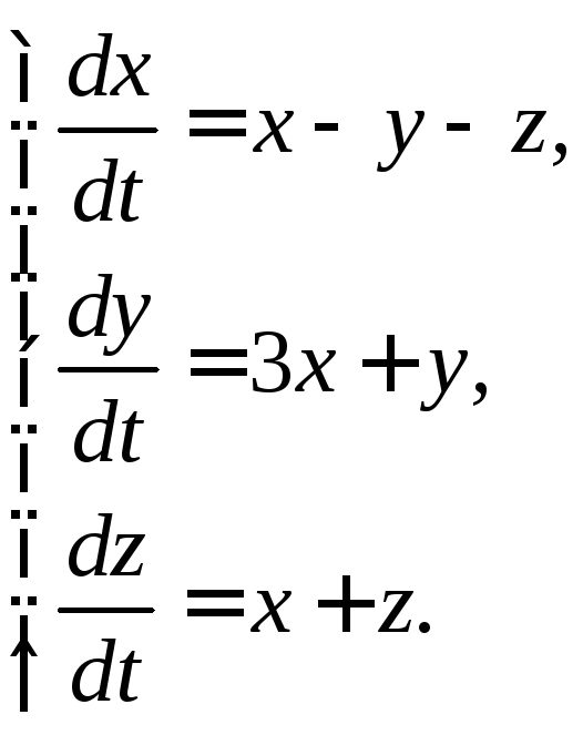
Consider, for example, a normal system of three equations with three unknown functions:

For a normal system of differential equations, the Cauchy theorem of the existence and uniqueness of a solution is formulated as follows.

Theorem. Let the right-hand sides of the equations of system (97), i.e., the functions are continuous in all variables in some domain G and have continuous partial derivatives in it.Then, whatever the values belonging to the domain G, there is a unique solution to the system satisfying the initial conditions:

To integrate system (97), one can apply a method by which this system, which contains three equations for three required functions, is reduced to one third-order equation with respect to one unknown function. Let us show an example of the application of this method.

For simplicity, we restrict ourselves to a system of two equations. Let a system of equations be given

To find a solution to the system, we proceed as follows. Differentiating the first of the equations of the system with respect to find

Substituting into this equality the expression from the second equation of the system, we obtain

Finally, replacing the function y by its expression from the first equation of the system

we obtain a linear homogeneous second-order equation with respect to one unknown function:

Integrating this equation, we find its general solution

Differentiating the equality, we find

Substituting expressions for x and into equality and reducing similar terms, we obtain

are the solution to this system.

So, integrating the normal system of two differential equations, we got its solution depending on two arbitrary constants.It can be shown that in the general case for a normal system consisting of equations, its general solution will depend on arbitrary constants.

Many systems of differential equations, both homogeneous and inhomogeneous, can be reduced to one equation for one unknown function. Let's show the method with examples.

Example 3.1. Solve system

Solution. 1) Differentiating by t first equation and using the second and third equations to replace and , we find

The resulting equation is differentiable with respect to again

1) Build the system

From the first two equations of the system, we express the variables and across
:

Substitute the found expressions for and in the third equation of the system

So, to find the function
obtained a differential equation of the third order with constant coefficients

2) We integrate the last equation by the standard method: we compose the characteristic equation
, find its roots
and construct a general solution in the form of a linear combination of exponentials, taking into account the multiplicity of one of the roots :.

3) Next, to find the two remaining functions
and
, we differentiate the twice obtained function

Using connections (3.1) between the functions of the system, we recover the remaining unknowns

Answer. ,
,.

It may turn out that all known functions except one are excluded from the third-order system already with a single differentiation. In this case, the order of the differential equation for finding it will be less than the number of unknown functions in the original system.

Example 3.2. Integrate the system

(3.2)

Solution. 1) Differentiating by the first equation, we find

Excluding variables and from equations

we will have a second-order equation with respect to

(3.3)

2) From the first equation of system (3.2) we have

(3.4)

Substituting the found expressions (3.3) and (3.4) for and , we obtain a first-order differential equation to determine the function

Integrating this inhomogeneous equation with constant first-order coefficients, we find
Using (3.4), we find the function

Answer.
,,
.

Task 3.1. Solve homogeneous systems by reducing to one differential equation.

3.1.1. 3.1.2.

3.1.3. 3.1.4.

3.1.5. 3.1.6.

3.1.7. 3.1.8.

3.1.9. 3.1.10.

3.1.11. 3.1.12.

3.1.13. 3.1.14.

3.1.15. 3.1.16.

3.1.17. 3.1.18.

3.1.19. 3.1.20.

3.1.21. 3.1.22.

3.1.23. 3.1.24.

3.1.25. 3.1.26.

3.1.27. 3.1.28.

3.1.29.
3.1.30.

3.2. Solving systems of linear homogeneous differential equations with constant coefficients by finding a fundamental system of solutions

The general solution of a system of linear homogeneous differential equations can be found as a linear combination of the fundamental solutions of the system. In the case of systems with constant coefficients, the methods of linear algebra can be used to find fundamental solutions.

Example 3.3. Solve system

(3.5)

Solution. 1) Let's rewrite the system in matrix form

. (3.6)

2) We will seek a fundamental solution to the system in the form of a vector
... Substituting functions
in (3.6) and canceling out by , we get

, (3.7)

that is the number must be an eigenvalue of the matrix
and the vector the corresponding eigenvector.

3) It is known from the course in linear algebra that system (3.7) has a nontrivial solution if its determinant is zero

that is . From here we find the eigenvalues
.

4) Find the corresponding eigenvectors. Substituting into (3.7) the first value
, we obtain a system for finding the first eigenvector

From here we get a connection between unknowns
... It is enough for us to choose one non-trivial solution. Assuming
, then
, that is, the vector is eigenvalue
, and the vector of the function
a fundamental solution to a given system of differential equations (3.5). Similarly, when substituting the second root
in (3.7) we have the matrix equation for the second eigenvector
... Where do we get the connection between its components
... Thus, we have the second fundamental solution