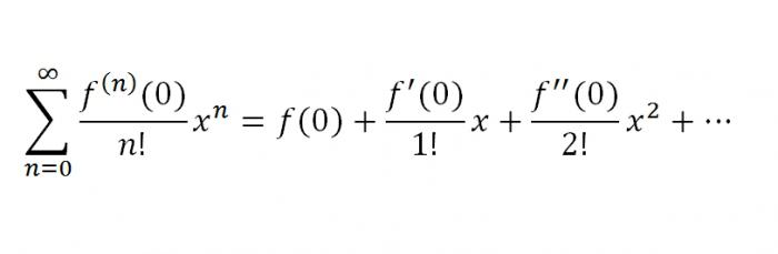
Taylor expansion formulas. Expansion of functions in power series

If the function f (x) has on some interval containing the point a, derivatives of all orders, then the Taylor formula can be applied to it:

where r n- the so-called remainder or the remainder of the series, it can be estimated using the Lagrange formula:

, where the number x is between NS and a.

If for some value x r n®0 for n® ¥, then in the limit the Taylor formula turns for this value into a convergent Taylor series:

So the function f (x) can be expanded into a Taylor series at the point under consideration NS, if:

1) it has derivatives of all orders;

2) the constructed series converges at this point.

At a= 0 we get a series called near Maclaurin:

Example 1 f (x) = 2x.

Solution... Let us find the values ​​of the function and its derivatives at NS=0

f (x) = 2x, f ( 0) = 2 0 =1;

f ¢ (x) = 2x ln2, f ¢ ( 0) = 2 0 ln2 = ln2;

f ¢¢ (x) = 2x ln 2 2, f ¢¢ ( 0) = 2 0 ln 2 2 = ln 2 2;

f (n) (x) = 2x ln n 2, f (n) ( 0) = 2 0 ln n 2 = ln n 2.

Substituting the obtained values ​​of the derivatives into the Taylor series formula, we get:

The radius of convergence of this series is equal to infinity; therefore, this expansion is valid for - ¥<x<+¥.

Example 2 NS+4) for the function f (x) = e x.

Solution... Find the derivatives of the function e x and their values ​​at the point NS=-4.

f (x)= e x, f (-4) = e -4 ;

f ¢ (x)= e x, f ¢ (-4) = e -4 ;

f ¢¢ (x)= e x, f ¢¢ (-4) = e -4 ;

f (n) (x)= e x, f (n) ( -4) = e -4 .

Therefore, the required Taylor series of the function has the form:

This expansion is also valid for - ¥<x<+¥.

Example 3 ... Expand function f (x)= ln x in a series in powers ( NS- 1),

(i.e., in the Taylor series in the vicinity of the point NS=1).

Solution... Find the derivatives of this function.

Substituting these values ​​into the formula, we get the required Taylor series:

Using the d'Alembert test, one can make sure that the series converges for

½ NS- 1½<1. Действительно,

The series converges if ½ NS- 1½<1, т.е. при 0<x<2. При NS= 2 we obtain an alternating series satisfying the conditions of the Leibniz test. At NS= 0 function is undefined. Thus, the domain of convergence of the Taylor series is the half-open interval (0; 2].

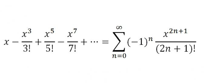
Let us present the expansions obtained in a similar way in the Maclaurin series (i.e., in the vicinity of the point NS= 0) for some elementary functions:

(2) ,

(3) ,

( the last decomposition is called binomial series)

Example 4 ... Expand a function in a power series

Solution... In expansion (1) we replace NS on - NS 2, we get:

Example 5 ... Expand the Maclaurin series function

Solution... We have

Using formula (4), we can write:

substituting for NS into the formula -NS, we get:

From here we find:

Expanding the brackets, rearranging the terms of the series and making a reduction of similar terms, we get

This series converges in the interval

(-1; 1), since it is obtained from two series, each of which converges in this interval.

Comment .

Formulas (1) - (5) can also be used to expand the corresponding functions in a Taylor series, i.e. for the expansion of functions in positive integer powers ( Ha). To do this, over a given function, it is necessary to perform such identical transformations in order to obtain one of the functions (1) - (5), in which, instead of NS costs k ( Ha) m, where k is a constant number, m is a positive integer. It is often convenient to change the variable t=Ha and expand the resulting function with respect to t in a Maclaurin series.

This method illustrates the theorem on the uniqueness of the expansion of a function in a power series. The essence of this theorem is that in the vicinity of the same point, two different power series cannot be obtained that would converge to the same function, no matter how its expansion is performed.

Example 6 ... Expand a function in a Taylor series in a neighborhood of a point NS=3.

Solution... This problem can be solved, as before, using the definition of the Taylor series, for which it is necessary to find the derivatives of the function and their values ​​at NS= 3. However, it will be easier to use the existing decomposition (5):

The resulting series converges for or –3<x- 3<3, 0<x< 6 и является искомым рядом Тейлора для данной функции.

Example 7 ... Write the Taylor series in powers ( NS-1) functions .

Solution.

The series converges at , or 2< x£ 5.

Students of higher mathematics should know that the sum of a certain power series belonging to the interval of convergence of the series given to us is a continuous and infinite number of times differentiated function. The question arises: is it possible to assert that a given arbitrary function f (x) is the sum of a certain power series? That is, under what conditions can f (x) be represented by a power series? The importance of such a question lies in the fact that it is possible to approximately replace the f-yu f (x) by the sum of the first few terms of the power series, that is, by a polynomial. This replacement of a function with a rather simple expression - a polynomial - is also convenient when solving some problems, namely: when solving integrals, when calculating, etc.

It is proved that for some f-u and f (x), in which it is possible to calculate the derivatives up to the (n + 1) th order, including the latter, in the neighborhood (α - R; x 0 + R) of some point x = α it is valid formula:

This formula bears the name of the famous scientist Brook Taylor. The series that is obtained from the previous one is called the Maclaurin series:

The rule that makes it possible to perform the expansion in the Maclaurin series:

1. Determine the derivatives of the first, second, third ... orders.
2. Calculate what the derivatives at x = 0 are equal to.
3. Write down the Maclaurin series for this function, and then determine the interval of its convergence.
4. Determine the interval (-R; R), where the residual part of the Maclaurin formula

R n (x) -> 0 as n -> infinity. If such exists, in it the function f (x) must coincide with the sum of the Maclaurin series.

Let us now consider the Maclaurin series for individual functions.

1. So, the first will be f (x) = e x. Of course, by its features, such a function has derivatives of various orders, and f (k) (x) = e x, where k is equal to all. Substitute x = 0. We get f (k) (0) = e 0 = 1, k = 1,2 ... Based on the above, the row e x will look like this:

2. Maclaurin series for the function f (x) = sin x. Let us clarify right away that the f-s for all unknowns will have derivatives, besides f "(x) = cos x = sin (x + n / 2), f" "(x) = -sin x = sin (x + 2 * n / 2) ..., f (k) (x) = sin (x + k * n / 2), where k is equal to any natural number.That is, making simple calculations, we can come to the conclusion that the series for f (x) = sin x will be of this form:

3. Now let's try to consider f-yu f (x) = cos x. For all unknowns, it has derivatives of arbitrary order, and | f (k) (x) | = | cos (x + k * n / 2) |<=1, k=1,2... Снова-таки, произведя определенные расчеты, получим, что ряд для f(х) = cos х будет выглядеть так:

So, we have listed the most important functions that can be expanded into a Maclaurin series, but they are supplemented by Taylor series for some functions. Now we will list them as well. It is also worth noting that the Taylor and Maclaurin series are an important part of the workshop for solving series in higher mathematics. So, the Taylor ranks.

1. The first will be the series for f-ii f (x) = ln (1 + x). As in the previous examples, for a given f (x) = ln (1 + x), we can add the series using the general form of the Maclaurin series. however, the Maclaurin series can be obtained much more simply for this function. Having integrated a certain geometric series, we get a series for f (x) = ln (1 + x) of such a sample:

2. And the second, which will be final in our article, will be the series for f (x) = arctan x. For x belonging to the interval [-1; 1], the decomposition is valid:

That's all. This article examined the most used Taylor and Maclaurin series in higher mathematics, in particular, in economics and technical universities.

How to embed mathematical formulas on a website?

If you ever need to add one or two mathematical formulas to a web page, then the easiest way to do this is as described in the article: mathematical formulas are easily inserted into the site in the form of pictures that Wolfram Alpha automatically generates. In addition to simplicity, this versatile method will help improve your site's visibility in search engines. It has been working for a long time (and I think it will work forever), but it is already outdated morally.

If you regularly use math formulas on your site, then I recommend that you use MathJax, a special JavaScript library that displays math notation in web browsers using MathML, LaTeX, or ASCIIMathML markup.

There are two ways to start using MathJax: (1) with a simple code, you can quickly connect a MathJax script to your site, which will be automatically loaded from a remote server at the right time (server list); (2) upload the MathJax script from a remote server to your server and connect it to all pages of your site. The second method, which is more complicated and time-consuming, will speed up the loading of your site's pages, and if the parent MathJax server for some reason becomes temporarily unavailable, this will not affect your own site in any way. Despite these advantages, I chose the first method as it is simpler, faster and does not require technical skills. Follow my example, and in 5 minutes you will be able to use all the features of MathJax on your site.

You can connect the script of the MathJax library from a remote server using two versions of the code taken from the main MathJax site or from the documentation page:

One of these code variants must be copied and pasted into the code of your web page, preferably between the tags and or right after the tag ... According to the first option, MathJax loads faster and slows down the page less. But the second option automatically tracks and loads the latest versions of MathJax. If you insert the first code, then it will need to be updated periodically. If you insert the second code, the pages will load more slowly, but you will not need to constantly monitor MathJax updates.

The easiest way to connect MathJax is in Blogger or WordPress: in your site's dashboard, add a widget designed to insert third-party JavaScript code, copy the first or second version of the loading code presented above into it, and place the widget closer to the beginning of the template (by the way, this is not necessary at all because the MathJax script is loaded asynchronously). That's all. Now, learn the MathML, LaTeX, and ASCIIMathML markup syntax, and you're ready to embed math formulas into your website's web pages.

Any fractal is built according to a certain rule, which is consistently applied an unlimited number of times. Each such time is called an iteration.

The iterative algorithm for constructing the Menger sponge is quite simple: the original cube with side 1 is divided by planes parallel to its faces into 27 equal cubes. One central cube and 6 adjacent cubes are removed from it. The result is a set consisting of the remaining 20 smaller cubes. Doing the same with each of these cubes, we get a set, already consisting of 400 smaller cubes. Continuing this process endlessly, we get a Menger sponge.

16.1. Expansion of elementary functions in Taylor series and

Maclaurin

Let us show that if an arbitrary function is defined on the set
, in the vicinity of the point
has many derivatives and is the sum of a power series:

then the coefficients of this series can be found.

Substitute in the power series
... Then
.

Find the first derivative of the function
:

At
:
.

For the second derivative we get:

At
:
.

Continuing this procedure n once we get:
.

Thus, we got a power series of the form:

,

which is called next to taylor for function
in the vicinity of the point
.

A special case of the Taylor series is Maclaurin series at
:

The remainder of the Taylor (Maclaurin) series is obtained by discarding from the main rows n first members and denoted as
... Then the function
can be written as the sum n early members of a number
and the remainder
:,

.

The remainder is usually
expressed in different formulas.

One of them is in the form of Lagrange:

, where
.
.

Note that in practice, the Maclaurin series is used more often. Thus, in order to write the function
in the form of a sum of a power series, it is necessary:

1) find the coefficients of the Maclaurin (Taylor) series;

2) find the region of convergence of the obtained power series;

3) prove that the given series converges to the function
.

Theorem1 (a necessary and sufficient condition for the convergence of the Maclaurin series). Let the radius of convergence of the series
... In order for this series to converge in the interval
to function
, it is necessary and sufficient for the condition to be satisfied:
in the specified interval.

Theorem 2. If the derivatives of any order of the function
in some interval
limited in absolute value by the same number M, that is
, then in this interval the function
can be expanded into a Maclaurin series.

Example1 . Expand in a Taylor row around the point
function.

Solution.

.

,;

,
;

,
;

,

.......................................................................................................................................

,
;

Convergence region
.

Example2 . Expand function in Taylor's row around the point
.

Solution:

Find the value of the function and its derivatives at
.

,
;

,
;

...........……………………………

,
.

We substitute these values ​​in a row. We get:

or
.

Let us find the region of convergence of this series. According to the d'Alembert feature, the series converges if

.

Therefore, for any this limit is less than 1, and therefore the region of convergence of the series will be:
.

Let us consider several examples of expansion in Maclaurin series of basic elementary functions. Recall that the Maclaurin series:

.

converges on the interval
to function
.

Note that in order to expand the function in a series, it is necessary:

a) find the coefficients of the Maclaurin series for this function;

b) calculate the radius of convergence for the resulting series;

c) prove that the resulting series converges to the function
.

Example 3. Consider the function
.

Solution.

Let us calculate the value of the function and its derivatives at
.

Then the numerical coefficients of the series are:

for anyone n. Substitute the found coefficients into the Maclaurin series and get:

Find the radius of convergence of the resulting series, namely:

.

Consequently, the series converges on the interval
.

This series converges to the function for any values because any gap
function and its derivatives in absolute value are limited by the number .

Example4 . Consider the function
.

Solution.

:

It is easy to see that the derivatives of even order
, and the derivatives are of odd order. We substitute the found coefficients into the Maclaurin series and obtain the expansion:

Let us find the interval of convergence of this series. On the basis of d'Alembert:

for anyone ... Consequently, the series converges on the interval
.

This series converges to the function
, because all its derivatives are limited to one.

Example5 .
.

Solution.

Let us find the value of the function and its derivatives at
:

Thus, the coefficients of this series:
and
, hence:

Similarly with the previous series, the region of convergence
... The series converges to the function
, because all its derivatives are limited to one.

Note that the function
odd and series expansion in odd powers, the function
- even and series expansion in even powers.

Example6 . Binomial series:
.

Solution.

Let us find the value of the function and its derivatives at
:

From this it is clear that:

Substitute these values ​​of the coefficients in the Maclaurin series and get the expansion of this function in a power series:

Find the radius of convergence of this series:

Consequently, the series converges on the interval
... At the limit points at
and
the series may or may not converge depending on the exponent
.

The series under study converges on the interval
to function
, that is, the sum of the charge
at
.

Example7 . Let us expand in a Maclaurin series the function
.

Solution.

To expand this function in series, we use the binomial series for
... We get:

Based on the property of power series (the power series can be integrated in the region of its convergence), we find the integral of the left and right sides of this series:

Find the region of convergence of this series:
,

that is, the region of convergence of this series is the interval
... Let us define the convergence of the series at the ends of the interval. At

... This row is a harmonious row, that is, it diverges. At
we get a number series with a common term
.

The Leibniz series converges. Thus, the region of convergence of this series is the interval
.

16.2. Applying Power Series in Approximate Calculations

In approximate calculations, power series play an extremely important role. With their help, tables of trigonometric functions, tables of logarithms, tables of values ​​of other functions were compiled, which are used in various fields of knowledge, for example, in probability theory and mathematical statistics. In addition, the expansion of functions in a power series is useful for their theoretical study. The main issue when using power series in approximate calculations is the issue of estimating the error when replacing the sum of a series with the sum of its first n members.

Consider two cases:

the function is expanded into alternating series;

the function is expanded into a constant series.

Calculation using alternating series

Let the function
expanded into an alternating power series. Then, when calculating this function for a specific value we obtain a numerical series to which the Leibniz test can be applied. In accordance with this feature, if the sum of the series is replaced by the sum of its first n terms, then the absolute error does not exceed the first term of the remainder of this series, that is:
.

Example8 . Calculate
accurate to 0.0001.

Solution.

We will use the Maclaurin series for
, substituting the value of the angle in radians:

If we compare the first and second terms of the series with a given accuracy, then:.

The third term of expansion:

less than the specified computation accuracy. Therefore, to calculate
it is enough to leave two members of the series, that is

.

Thus
.

Example9 . Calculate
with an accuracy of 0.001.

Solution.

We will use the binomial series formula. To do this, write
as:
.

In this expression
,

Let's compare each of the members of the series with the specified accuracy. It's clear that
... Therefore, to calculate
it is enough to leave three members of the row.

or
.

Calculation using positive series

Example10 . Calculate the number accurate to 0.001.

Solution.

In a row for the function
substitute
... We get:

Let us estimate the error that arises when the sum of the series is replaced by the sum of the first members. Let's write down the obvious inequality:

that is 2<<3. Используем формулу остаточного члена ряда в форме Лагранжа:
,
.

According to the condition of the problem, you need to find n such that the following inequality holds:
or
.

It is easy to check that for n= 6:
.

Hence,
.

Example11 . Calculate
with an accuracy of 0.0001.

Solution.

Note that to calculate the logarithms, one could apply a series for the function
, but this series converges very slowly and 9999 terms would have to be taken to achieve the specified accuracy! Therefore, to calculate logarithms, as a rule, a series for the function is used
which converges on the interval
.

Let's calculate
using this row. Let be
, then .

Hence,
,

In order to calculate
with a given accuracy, we take the sum of the first four terms:
.

Remainder of the row
discard. Let's estimate the error. It's obvious that

or
.

Thus, in the series that was used for the calculation, it was enough to take only the first four terms instead of 9999 in the series for the function
.

Self-test questions

1. What is a Taylor series?

2. What kind did the Maclaurin series have?

3. Formulate a theorem on the expansion of a function in a Taylor series.

4. Write the Maclaurin series expansion of the main functions.

5. Indicate the regions of convergence of the series considered.

6. How to estimate the error in approximate calculations using power series?

If the function f (x) has derivatives of all orders on some interval containing the point a, then the Taylor formula can be applied to it:
,
where r n- the so-called remainder or the remainder of the series, it can be estimated using the Lagrange formula:
, where the number x is between x and a.

f (x) =

At the point x 0 =
Number of elements in a row 3 4 5 6 7
Use the expansion of elementary functions e x, cos (x), sin (x), ln (1 + x), (1 + x) m

Function entry rules:

If for some value NS r n→ 0 for n→ ∞, then in the limit the Taylor formula turns for this value into a convergent Taylor series:
,
Thus, the function f (x) can be expanded in a Taylor series at the considered point x if:
1) it has derivatives of all orders;
2) the constructed series converges at this point.

For a = 0, we obtain a series called near Maclaurin:
,
Expansion of the simplest (elementary) functions in the Maclaurin series:
Indicative functions
, R = ∞
Trigonometric functions
, R = ∞
, R = ∞
, (-π / 2< x < π/2), R=π/2
The actgx function does not expand in powers of x, since ctg0 = ∞
Hyperbolic functions


Logarithmic functions
, -1
Binomial series
.

Example # 1. Expand a function in a power series f (x) = 2x.
Solution... Let us find the values ​​of the function and its derivatives at NS=0
f (x) = 2x, f ( 0) = 2 0 =1;
f "(x) = 2x ln2, f "( 0) = 2 0 ln2 = ln2;
f "" (x) = 2x ln 2 2, f "" ( 0) = 2 0 ln 2 2 = ln 2 2;
…
f (n) (x) = 2x ln n 2, f (n) ( 0) = 2 0 ln n 2 = ln n 2.
Substituting the obtained values ​​of the derivatives into the formula of the Taylor series, we get:

The radius of convergence of this series is equal to infinity, so this expansion is valid for -∞<x<+∞.

Example # 2. Write the Taylor series in powers ( NS+4) for the function f (x) = e x.
Solution... Find the derivatives of the function e x and their values ​​at the point NS=-4.
f (x)= e x, f (-4) = e -4 ;
f "(x)= e x, f "(-4) = e -4 ;
f "" (x)= e x, f "" (-4) = e -4 ;
…
f (n) (x)= e x, f (n) ( -4) = e -4 .
Therefore, the required Taylor series of the function has the form:

This decomposition is also valid for -∞<x<+∞.

Example No. 3. Expand function f (x)= ln x in a series in powers ( NS- 1),
(i.e., in the Taylor series in the vicinity of the point NS=1).
Solution... Find the derivatives of this function.
f (x) = lnx,,,,

f (1) = ln1 = 0, f "(1) = 1, f" "(1) = - 1, f" "" (1) = 1 * 2, ..., f (n) = (- 1) n-1 (n-1)!
Substituting these values ​​into the formula, we get the required Taylor series:

Using the d'Alembert test, one can make sure that the series converges for ½x-1½<1 . Действительно,

The series converges if ½ NS- 1½<1, т.е. при 0<x<2. При NS= 2 we obtain an alternating series satisfying the conditions of the Leibniz test. For x = 0, the function is undefined. Thus, the domain of convergence of the Taylor series is the half-open interval (0; 2].

Example No. 4. Expand the function in a power series.
Solution... In the expansion (1) we replace x by -x 2, we get:
, -∞

Example No. 5. Expand the Maclaurin function.
Solution... We have
Using formula (4), we can write:

substituting instead of x in the formula -x, we get:

From here we find: ln (1 + x) -ln (1-x) = -
Expanding the brackets, rearranging the terms of the series and making a reduction of similar terms, we get
... This series converges in the interval (-1; 1), since it is obtained from two series, each of which converges in this interval.

Comment .
Formulas (1) - (5) can also be used to expand the corresponding functions in a Taylor series, i.e. for the expansion of functions in positive integer powers ( Ha). To do this, over a given function, it is necessary to perform such identical transformations in order to obtain one of the functions (1) - (5), in which, instead of NS costs k ( Ha) m, where k is a constant number, m is a positive integer. It is often convenient to change the variable t=Ha and expand the resulting function with respect to t in a Maclaurin series.

This method is based on the uniqueness theorem for the expansion of a function in a power series. The essence of this theorem is that in the vicinity of the same point, two different power series cannot be obtained that would converge to the same function, no matter how its expansion is performed.

Example No. 5a. Expand the function in a Maclaurin series, indicate the region of convergence.
Solution. First, find 1-x-6x 2 = (1-3x) (1 + 2x),.
to elementary:

The fraction 3 / (1-3x) can be viewed as the sum of an infinitely decreasing geometric progression with the denominator 3x, if | 3x |< 1. Аналогично, дробь 2/(1+2x) как сумму бесконечно убывающей геометрической прогрессии знаменателем -2x, если |-2x| < 1. В результате получим разложение в степенной ряд

with the region of convergence | x |< 1/3.

Example No. 6. Expand the function in a Taylor series in the vicinity of the point x = 3.
Solution... This problem can be solved, as before, using the definition of the Taylor series, for which it is necessary to find the derivatives of the function and their values ​​at NS= 3. However, it will be easier to use the existing decomposition (5):
=
The resulting series converges at or –3

Example No. 7. Write the Taylor series in powers (x -1) of the function ln (x + 2).
Solution.


The series converges at, or -2< x < 5.

Example No. 8. Expand the function f (x) = sin (πx / 4) in a Taylor series in the vicinity of the point x = 2.
Solution... Let's make the substitution t = x-2:

Using expansion (3), in which we substitute π / 4 t in place of x, we obtain:

The resulting series converges to a given function at -∞< π / 4 t<+∞, т.е. при (-∞Thus,
, (-∞

Approximate Calculations Using Power Series

Power series are widely used in approximate calculations. With their help, with a given accuracy, you can calculate the values ​​of roots, trigonometric functions, logarithms of numbers, definite integrals. The series are also used when integrating differential equations.
Consider the expansion of a function in a power series:

In order to calculate the approximate value of the function at a given point NS belonging to the region of convergence of the indicated series, the first n members ( n Is a finite number), and the remaining terms are discarded:

To estimate the error of the obtained approximate value, it is necessary to estimate the discarded remainder r n (x). For this, the following techniques are used:

• if the resulting series is alternating with signs, then the following property is used: for an alternating series satisfying the Leibniz conditions, the remainder of the series in absolute value does not exceed the first discarded term.
• if a given row is constant in sign, then a row composed of discarded members is compared with an infinitely decreasing geometric progression.
• in the general case, to estimate the remainder of the Taylor series, one can use the Lagrange formula: a x ).

Example # 1. Calculate ln (3) to the nearest 0.01.
Solution... Let's use the expansion, where x = 1/2 (see example 5 in the previous topic):

Let's check if we can discard the remainder after the first three terms of the expansion, for this we estimate it using the sum of an infinitely decreasing geometric progression:

So we can discard this remainder and get

Example # 2. Calculate to the nearest 0.0001.
Solution... Let's use the binomial series. Since 5 3 is the closest cube of an integer to 130, it is advisable to represent the number 130 as 130 = 5 3 +5.



since already the fourth term of the obtained alternating series satisfying the Leibniz criterion is less than the required accuracy:
, therefore, it and the members following it can be discarded.
Many practically necessary definite or improper integrals cannot be calculated using the Newton-Leibniz formula, because its application is associated with finding an antiderivative, which often does not have an expression in elementary functions. It also happens that finding the antiderivative is possible, but unnecessarily laborious. However, if the integrand can be expanded into a power series, and the limits of integration belong to the interval of convergence of this series, then an approximate calculation of the integral with a predetermined accuracy is possible.

Example No. 3. Evaluate integral ∫ 0 1 4 sin (x) x to the nearest 10 -5.
Solution... The corresponding indefinite integral cannot be expressed in elementary functions, i.e. is an "unbreakable integral". It is impossible to apply the Newton-Leibniz formula here. Let us calculate the integral approximately.
By dividing the series for sin x on x, we get:

Integrating this series term by term (this is possible, since the limits of integration belong to the interval of convergence of this series), we obtain:

Since the resulting series satisfies Leibniz's conditions, it is enough to take the sum of the first two terms to get the desired value with a given accuracy.
Thus, we find
.

Example No. 4. Evaluate the integral ∫ 0 1 4 e x 2 to the nearest 0.001.
Solution.
... Let's check if we can discard the remainder after the second term of the resulting series.
0.0001<0.001. Следовательно, .