Variational and statistical distribution series. Variational Series Analysis
An example of solving a test on mathematical statistics
Problem 1
Initial data : students of a certain group of 30 people passed the exam in the course "Informatics". The grades received by the students form the following series of numbers:
I. Let's compose a variation series
|
m x |
w x |
m x nak |
w x nak |
|
|
Total: |
II. Graphical presentation of statistical information.

III. Numerical characteristics of the sample.
1. Arithmetic mean
2. Geometric mean
3. Fashion 
4. Median
222222333333333 | 3 34444444445555

5. Sample variance

7. Coefficient of variation

8. Asymmetry
9. Asymmetry coefficient

10. Excess
11. The coefficient of kurtosis

Task 2
Initial data : students of a certain group wrote their final test. The group consists of 30 people. The points scored by the students form the following series of numbers
Solution
I. Since the feature takes on many different values, we will construct an interval variation series for it. To do this, first set the value of the interval h... We will use Stairger's formula
Let's compose a scale of intervals. In this case, we will take the value determined by the formula for the upper boundary of the first interval:
The upper bounds of the subsequent intervals are determined by the following recursive formula:
 , then
We finish building the scale of intervals, since the upper limit of the next interval has become greater than or equal to the maximum value of the sample  .
.
|
|
|
|
|
|


II. Graphical display of interval variation series


III. Numerical characteristics of the sample
To determine the numerical characteristics of the sample, we will compose an auxiliary table
|
|
|
|
|
|
|
|
Sum: |


1. Arithmetic mean

2. Geometric mean
3. Fashion 
4. Median
10 11 12 12 13 13 13 13 14 14 14 14 15 15 15 |15 15 15 16 16 16 16 16 17 17 18 19 19 20 20

5. Sample variance

6. Sample standard deviation

7. Coefficient of variation

8. Asymmetry

9. Asymmetry coefficient

10. Excess

11. The coefficient of kurtosis

Problem 3
Condition : the scale division of the ammeter is 0.1 A. Readings are rounded to the nearest whole division. Find the probability that an error exceeding 0.02 A.
Solution.
The rounding error can be considered as a random value. X, which is distributed evenly in the interval between two adjacent integer divisions. Density of uniform distribution
 ,
,
where  - the length of the interval in which the possible values are enclosed X; outside this interval
  In this problem, the length of the interval containing the possible values X, is equal to 0.1, therefore

The counting error will exceed 0.02 if it is enclosed in the interval (0.02; 0.08). Then
Answer: R=0,6
Problem 4
Initial data: mathematical expectation and standard deviation of a normally distributed feature X are, respectively, 10 and 2. Find the probability that in the test result X will take the value enclosed in the interval (12, 14).
Solution.
Let's use the formula

And theoretical frequencies 


For X her expected value M (X) and variance D (X). Solution... Find the distribution function F (x) random variable... sampling error). Let's compose variational row Span Width will be: For each value a number of let's calculate how many ...
Solution: Separable Equation
SolutionIn the form To find the private solutions inhomogeneous equation make up system Let's solve the resulting system ...; +47; +61; +10; -eight. Construct Interval variational row... Give statistical estimates average ...
Solution: Let's calculate chain and basic absolute increments, growth rates, growth rates. The obtained values are summarized in table 1
SolutionProduction volume. Solution: Arithmetic mean of interval variational a number of is calculated as follows: for ... The marginal sampling error with a probability of 0.954 (t = 2) will be: Δ w = t * μ = 2 * 0.0146 = 0.02927 Determine the boundaries ...
Solution. Sign
SolutionAbout whose work experience and made up sample. The sample average length of time ... of the working day of these employees and made up sample. The average duration for the sample is ... 1.16, the significance level is α = 0.05. Solution. Variational row of this sample has the form: 0.71 ...
Working curriculum in biology for grades 10-11 Compiled by S. Polikarpova
Working curriculumThe simplest crossing schemes "5 LR. " Solution elementary genetic problems "6 L. r. " Solution elementary genetic problems ”7 L. r. “..., 110, 115, 112, 110. Make up variational row, draw variational curve, find the average value of the feature ...
(definition of the variation series; components of the variation series; three forms of the variation series; expediency of constructing an interval series; conclusions that can be drawn from the constructed series)
The variation series is the sequence of all the elements of the sample, arranged in a non-decreasing order. Identical elements are repeated
Variational ones are series built on a quantitative basis.
Variational distribution series consist of two elements: options and frequencies:
Variants are the numerical values of a quantitative characteristic in the variation series of the distribution. They can be positive and negative, absolute and relative. So, when grouping enterprises according to the results of economic activity, the positive options are profit, and negative numbers Is a loss.
Frequencies are the numbers of individual variants or each group of the variation series, i.e. these are numbers showing how often one or another variant occurs in a distribution series. The sum of all frequencies is called the volume of the population and is determined by the number of elements of the entire population.
Frequencies are frequencies expressed as relative values (fractions of units or percentages). The sum of the frequencies is equal to one or 100%. Replacing frequencies with frequencies allows one to compare the series of variations with a different number of observations.
There are three forms of the variation series: ranked range, discrete range and interval range.
A ranked series is the distribution of individual units of a population in ascending or descending order of the trait under study. Ranking allows you to easily divide quantitative data into groups, immediately find the smallest and largest values of a feature, highlight the values that are most often repeated.
Other forms of the variation series are group tables compiled according to the nature of the variation in the values of the trait under study. By the nature of the variation, discrete (discontinuous) and continuous signs are distinguished.
Discrete series is a variation series based on features with discontinuous change (discrete features). The latter include tariff category, the number of children in the family, the number of employees at the enterprise, etc. These characteristics can only take on a finite number of specific values.
A discrete variation series is a table that consists of two graphs. The first column indicates the specific value of the attribute, and the second - the number of units of the population with a specific value of the attribute.
If a feature has a continuous change (income, work experience, the cost of fixed assets of the enterprise, etc., which within certain limits can take any values), then for this feature it is necessary to build an interval variation series.
The group table also has two columns here. The first contains the value of the feature in the interval "from - to" (options), the second - the number of units included in the interval (frequency).
Frequency (repetition rate) - the number of repetitions of a separate variant of the attribute values, denoted by fi, and the sum of frequencies equal to the volume of the studied population is denoted
Where k is the number of options for characteristic values
Very often, the table is supplemented with a column in which the accumulated frequencies S are calculated, which show how many units of the population have a feature value no more than a given value.
A discrete variation series of a distribution is a series in which groups are composed according to a feature that changes discretely and takes only integer values.
An interval variation series of a distribution is a series in which the grouping attribute that forms the basis of the grouping can take any values in a certain interval, including fractional ones.
Interval variation series an ordered set of intervals of variation of the values of a random variable with the corresponding frequencies or frequencies of occurrence of values of the quantity in each of them is called.
Interval series It is advisable to construct distributions, first of all, with continuous variation of a feature, and also if discrete variation manifests itself in wide limits, i.e. number of options discrete feature big enough.
Several conclusions can already be drawn from this series. For example, the mean of the variation series (median) can be an estimate of the most likely measurement result. The first and last element of the variation series (i.e., the minimum and maximum sample unit) show the dispersion of the sample items. Sometimes, if the first or last element is very different from the rest of the sample, then they are excluded from the measurement results, considering that these values were obtained as a result of some gross failure, for example, technology.
Statistical distribution series- This is an ordered distribution of units of the population into groups according to a certain varying characteristic.Depending on the feature underlying the formation of a distribution series, there are attributive and variation series of distribution.
The presence of a common feature is the basis for the formation of a statistical population, which is the results of description or measurement common features objects of research.
The subject of study in statistics is changing (varying) signs or statistical signs.
Types of statistical signs.
Distribution series are called attributive based on quality criteria. Attributive Is a sign that has a name (for example, profession: seamstress, teacher, etc.).
It is customary to arrange a number of distributions in the form of tables. Table 2.8 shows the attributive series of distribution.
Table 2.8 - Distribution of types of legal assistance provided by lawyers to citizens of one of the regions of the Russian Federation.
The distribution series are called variation series built on a quantitative basis. Any variation series consists of two elements: options and frequencies.
Variants are considered to be the individual values of the characteristic that it takes in the variation series.
Frequencies are the numbers of individual variants or each group of the variation series, i.e. these are numbers showing how often one or another variant occurs in a distribution series. The sum of all frequencies determines the number of the entire population, its volume.
Frequencies are frequencies expressed in fractions of one or as a percentage of the total. Accordingly, the sum of the frequencies is 1 or 100%. The series of variations allows us to estimate the shape of the distribution law using actual data.
Depending on the nature of the variation of the trait, they are distinguished discrete and interval variation series.
An example of a discrete variation series is given in table. 2.9.
Table 2.9 - Distribution of families by the number of occupied rooms in separate apartments in 1989 in the Russian Federation.
Variational series
V the general population some quantitative feature is being investigated. A sample of volume is randomly extracted from it n, that is, the number of elements in the sample is n... At the first stage of statistical processing, ranging sampling, i.e. ordering numbers x 1, x 2, ..., x n Ascending. Each observed value x i called variant... Frequency m i Is the number of observations of the value x i in the sample. Relative frequency (frequency) w i Is the frequency ratio m i to the sample size n: .When studying the variation series, the concepts of accumulated frequency and accumulated frequency are also used. Let x some number. Then the number of options , whose values are less x, is called the accumulated frequency: for x i
A feature is called discretely varied if its individual values (variants) differ from each other by some finite value (usually an integer). The variation series of such a feature is called a discrete variation series.
Table 1. General view of the discrete variation series of frequencies
| Characteristic values | x i | x 1 | x 2 | … | x n |
| Frequencies | m i | m 1 | m 2 | … | m n |
A feature is called continuously varying if its values differ from each other by an arbitrarily small amount, i.e. the attribute can take on any values in a certain interval. A continuous variation series for such a feature is called interval.
Table 2. General view of the interval variation series of frequencies
Table 3. Graphic images of the variation series
| Row | Polygon or histogram | Empirical distribution function | |
| Discrete |  |  | 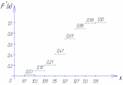 |
| Interval |  | 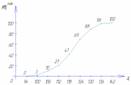 | 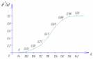 |
For graphical representation of variation series, polygon, histogram, cumulative curve and empirical distribution function are most often used.
Table 2.3 (Grouping of the population of Russia by average per capita income in April 1994) is presented interval variation series.
It is convenient to analyze distribution series with the help of a graphic image, which makes it possible to judge the shape of the distribution. A clear idea of the nature of the change in the frequencies of the variation series is given by polygon and histogram.
The polygon is used when displaying discrete variation series.
Let's depict, for example, graphically the distribution of the housing stock by type of apartments (Table 2.10).
Table 2.10 - Distribution of the housing stock of the urban area by type of apartments (arbitrary numbers).

Rice. Housing stock allocation polygon
On the ordinate axis, not only the values of frequencies, but also the frequencies of the variation series can be plotted.
The histogram is taken for the image of the interval variation series... When constructing a histogram, the values of the intervals are plotted on the abscissa axis, and the frequencies are depicted by rectangles built at the corresponding intervals. The height of the bars in the case of equal spacing should be proportional to the frequencies. A histogram is a graph in which a series is shown in the form of bars adjacent to each other.
Let us graphically depict the interval distribution series given in table. 2.11.
Table 2.11 - Distribution of families by the size of living space per person (arbitrary numbers).
| N p / p | Groups of families according to the size of living space per person | The number of families with a given size of living space | Accumulated number of families |
| 1 | 3 – 5 | 10 | 10 |
| 2 | 5 – 7 | 20 | 30 |
| 3 | 7 – 9 | 40 | 70 |
| 4 | 9 – 11 | 30 | 100 |
| 5 | 11 – 13 | 15 | 115 |
| TOTAL | 115 | ---- | |

Rice. 2.2. Histogram of the distribution of families by the size of living space per person
Using the data of the accumulated series (Table 2.11), we construct cumulative distribution.

Rice. 2.3. Cumulative distribution of families by living space per person
The representation of the variation series in the form of cumulates is especially effective for variation series, the frequencies of which are expressed in fractions or percentages to the sum of the frequencies of the series.
If we change the axes when graphically depicting the variation series in the form of cumulates, then we get ogive... In fig. 2.4 shows the ogive built on the basis of the data in Table. 2.11.
A histogram can be converted to a distribution polygon by finding the midpoints of the sides of the rectangles and then connecting these points with straight lines. The resulting distribution polygon is shown in Fig. 2.2 with a dotted line.
When constructing a histogram of the distribution of the variation series with unequal intervals on the ordinate axis, not the frequencies are plotted, but the density of the feature distribution in the corresponding intervals.
The distribution density is the frequency calculated per unit interval width, i.e. how many units are in each group per unit of the interval. An example of calculating the distribution density is presented in table. 2.12.
Table 2.12 - Distribution of enterprises by the number of employees (conditional numbers)
| N p / p | Groups of enterprises by the number of employees, people | Number of enterprises | Interval size, persons | Distribution density |
| A | 1 | 2 | 3=1/2 | |
| 1 | Up to 20 | 15 | 20 | 0,75 |
| 2 | 20 – 80 | 27 | 60 | 0,25 |
| 3 | 80 – 150 | 35 | 70 | 0,5 |
| 4 | 150 – 300 | 60 | 150 | 0,4 |
| 5 | 300 – 500 | 10 | 200 | 0,05 |
| TOTAL | 147 | ---- | ---- |
For graphical representation of the variation series can also be used cumulative curve... With the help of cumulates (sum curve), a series of accumulated frequencies is displayed. The accumulated frequencies are determined by sequentially summing up the frequencies by groups and show how many units of the population have a characteristic value no greater than the considered value.

Rice. 2.4. Range of distribution of families by the size of living space per person
When constructing the cumulates of the interval variation series, the variants of the series are plotted along the abscissa axis, and the accumulated frequencies are plotted along the ordinate axis.
Variational series - This is a statistical series showing the distribution of the phenomenon under study by the value of any quantitative attribute. For example, patients by age, by terms of treatment, newborns by weight, etc.
Option - individual values of the characteristic by which the grouping is carried out (denoted by V ) .
Frequency- a number showing how often one or another option occurs (denoted P ) ... The sum of all frequencies shows total number observations and denoted n ... The difference between the largest and smallest variants of the variation series is called swing or amplitude .
There are variation series:
1. Discontinuous (discrete) and continuous.
The series is considered continuous if the grouping attribute can be expressed in fractional quantities (weight, height, etc.), discontinuous, if the grouping attribute is expressed only as a whole number (days of disability, the number of heartbeats, etc.).
2.Simple and balanced.
A simple variation series is a series in which the quantitative value of a variable characteristic occurs once. In a weighted variation series, the quantitative values of a variable feature are repeated with a certain frequency.
3. Grouped (interval) and ungrouped.
A grouped row has options, combined into groups, combining them in size within a certain interval. In an ungrouped row, each individual variant corresponds to a certain frequency.
4. Even and odd.
In even series of variations, the sum of frequencies or the total number of observations is expressed in an even number, in odd ones - in an odd one.
5. Symmetrical and asymmetrical.
In a symmetric variation series, all kinds of means coincide or are very close (mode, median, arithmetic mean).
Depending on the nature of the studied phenomena, on the specific tasks and goals of statistical research, as well as on the content of the source material, in sanitary statistics the following types of averages apply:
structural averages (fashion, median);
arithmetic mean;
average harmonic;
geometric mean;
medium progressive.
Fashion (M O ) - the value of the variable characteristic, which is more often found in the studied population, i.e. option corresponding to the highest frequency. They find it directly from the structure of the variational series, without resorting to any calculations. It is usually a value very close to the arithmetic mean and is very convenient in practice.
Median (M e ) - dividing the variation series (ranked, i.e. the values of the variant are arranged in ascending or descending order) into two equal halves. The median is calculated using the so-called odd series, which is obtained by successively summing the frequencies. If the sum of the frequencies corresponds to an even number, then the arithmetic mean of the two mean values is conventionally taken as the median.
Mode and median apply in the case of an open population, i.e. when the largest or smallest options do not have an accurate quantitative characteristic (for example, up to 15 years old, 50 and older, etc.). In this case, the arithmetic mean (parametric characteristics) cannot be calculated.
Average i am arithmetic is the most common value. The arithmetic mean is denoted more often through M.
Distinguish between simple and weighted arithmetic mean.
Simple arithmetic mean calculated:
- in cases where the aggregate is represented by a simple list of knowledge of the attribute for each unit;
- if the number of repetitions of each option is not possible to determine;
- if the number of repetitions of each option is close to each other.
The simple arithmetic mean is calculated by the formula:
where V - individual values of the attribute; n is the number of individual values;  is the summation sign.
Thus, the simple average is the ratio of the sum of the variant to the number of observations.
Example: determine the average length of stay in bed for 10 patients with pneumonia:
16 days - 1 patient; 17-1; 18-1; 19-1; 20-1; 21-1; 22-1; 23-1; 26-1; 31-1.
bed-day.
Weighted arithmetic mean calculated in cases where the individual values of the characteristic are repeated. It can be calculated in two ways:
1. Direct (arithmetic mean or direct method) according to the formula:
 ,
,
where P is the frequency (number of cases) of observations of each option.
Thus, the weighted arithmetic mean is the ratio of the sum of the products of the variant by the frequency to the number of observations.
2. By calculating deviations from the conditional average (by the method of moments).
The basis for calculating the weighted arithmetic mean is:
- grouped material according to the variants of the quantitative attribute;
- all options should be arranged in ascending or descending order of the value of the feature (ranked series).
To calculate by the method of moments, a prerequisite is the same size of all intervals.
According to the method of moments, the arithmetic mean is calculated by the formula:
 ,
,
where M o is the conditional average, for which the value of the feature corresponding to the highest frequency is often taken, i.e. which repeats more often (Fashion).
i is the size of the interval.
a - conditional deviation from the conditions of the average, which is a sequential series of numbers (1, 2, etc.) with a + sign for the variant of large conditional average and with the sign - (- 1, –2, etc.) for the variant, which are below the conditional average. The conditional deviation from the options, taken as the conditional average, is equal to 0.
P - frequencies.
 - the total number of observations or n.
Example: determine the average height of boys 8 years old directly (table 1).
Table 1
|
Height in cm |
boys P |
Central option V | |
The central variant - the middle of the interval - is defined as the semi-sum of the initial values of two neighboring groups:
 ;
;  etc.
etc.
The VP product is obtained by multiplying the center variants by the frequencies  ;
; etc. Then the resulting products are added and received
  , which is divided by the number of observations (100) and the weighted arithmetic mean is obtained.
 cm.
cm.
We will solve the same problem by the method of moments, for which the following table 2 is compiled:
Table 2
|
Height in cm (V) |
boys P | ||
n = 100 
We take 122 as M o, since out of 100 observations, 33 people were 122cm tall. Find the conditional deviations (a) from the conditional average in accordance with the above. Then we obtain the product of the conditional deviations by the frequencies (aP) and sum the obtained values (  ). As a result, we get 17. Finally, we substitute the data into the formula:

When studying a variable characteristic, one cannot be limited only to the calculation of average values. It is also necessary to calculate indicators characterizing the degree of diversity of the studied characteristics. The value of this or that quantitative characteristic is not the same for all units of the statistical population.
The characteristic of the variation series is the standard deviation (  ), which shows the spread (dispersion) of the studied features relative to the arithmetic mean, i.e. characterizes the variability of the variation series. It can be determined directly by the formula:

The standard deviation is equal to the square root of the sum of the products of the squares of the deviations of each option from the arithmetic mean (V – M) 2 by its frequencies divided by the sum of frequencies (  ).
).
Calculation example: determine the average number of sick leaves issued in the clinic per day (table 3).
Table 3
|
Number of sick leave sheets issued doctor per day (V) |
Number of doctors (P) | ||||
 ;
; 
In the denominator, when the number of observations is less than 30, it is necessary from  subtract one.
If the series is grouped at equal intervals, then the standard deviation can be determined by the method of moments:
 ,
,
where i is the size of the interval;
 - conditional deviation from the conditional average;
P - frequency variant of the corresponding intervals;
 - the total number of observations.
Calculation example : Determine the average length of stay of patients in a therapeutic bed (by the method of moments) (table 4):
Table 4
|
Number of days stay in bed (V) |
sick (P) |
|
|
|


 ;
;
The Belgian statistician A. Quetelet discovered that variations in mass phenomena obey the law of distribution of errors, discovered almost simultaneously by K. Gauss and P. Laplace. The curve representing this distribution looks like a bell. According to the normal distribution law, the variability of the individual values of the trait is within the range  that covers 99.73% of all units of the population.
It is calculated that if we add and subtract 2 to the arithmetic mean  , then within the obtained values there are 95.45% of all members of the variation series and, finally, if we add and subtract 1 to the arithmetic mean
  , then within the obtained values will be 68.27% of all members of the given variation series. In medicine with magnitude
  1
1 the concept of the norm is connected. Deviation from the arithmetic mean by more than 1
  , but less than 2
  is subnormal, and the deviation is greater than 2
  abnormal (above or below normal).
In sanitary statistics, the three sigma rule is applied in the study of physical development, the assessment of the performance of health care institutions, and the assessment of the health of the population. The same rule is widely used in the national economy when defining standards.
Thus, the standard deviation serves to:
- measuring the variance of the variation series;
- characteristics of the degree of diversity of features, which are determined by the coefficient of variation:

If the coefficient of variation is more than 20% - a strong variety, from 20 to 10% - an average, less than 10% - a weak variety of traits. The coefficient of variation is, to a certain extent, a criterion for the reliability of the arithmetic mean.
Rows built quantitatively are called variational.
Distribution series consist of options(characteristic values) and frequencies(number of groups). Frequencies expressed as relative values (fractions, percentages) are called frequent... The sum of all frequencies is called the volume of the distribution series.
By type, the distribution series are divided into discrete(built on the basis of discontinuous values of the characteristic) and interval(built on continuous values of the characteristic).
Variational series represents two columns (or lines); in one of which the individual values of the variable attribute are given, referred to as options and denoted by X; and in the other - absolute numbers showing how many times (how often) each option occurs. The indicators of the second column are called frequencies and are conventionally denoted by f. Once again, we note that in the second column, relative indicators can also be used, characterizing the share of the frequency of individual variants in the total sum of frequencies. These relative indicators are called frequencies and are conventionally denoted through ω The sum of all the frequencies in this case is equal to one. However, frequencies can be expressed as a percentage, and then the sum of all frequencies gives 100%.
If the variants of the variation series are expressed in the form of discrete quantities, then such a variation series is called discrete.
For continuous features, the variational series are constructed as interval, that is, the values of the attribute in them are expressed "from ... to ...". At the same time, the minimum values of the attribute in such an interval are called the lower boundary of the interval, and the maximum - the upper boundary.
Interval variation series are also constructed for discrete features varying in a large range. Interval rows can be with equal and unequal intervals.
Consider how the value of equal intervals is determined. Let us introduce the following notation:
i- the size of the interval;
- the maximum value of the attribute for the units of the population;
- the minimum value of the characteristic for the units of the population;
n - the number of allocated groups.
if n is known.
If the number of allocated groups is difficult to determine in advance, then the formula proposed by Sturgess in 1926 can be recommended for calculating the optimal value of the interval with a sufficient volume of the population:
n = 1+ 3.322 lg N, where N is the number of units in the aggregate.
The size of the unequal intervals is determined in each individual case, taking into account the characteristics of the object of study.
Statistical distribution of the sample call a list of options and their corresponding frequencies (or relative frequencies).
The statistical distribution of the sample can be set in the form of a table, in the first column of which the options are located, and in the second - the frequencies corresponding to these options ni, or relative frequencies Pi .
Statistical distribution of the sample
Variation series are called interval series, in which the values of the characteristics underlying their formation are expressed within certain limits (intervals). Frequencies in this case refer not to individual characteristic values, but to the entire interval.
Interval distribution series are built according to continuous quantitative features, as well as discrete features varying within significant limits.
The interval series can be represented by the statistical distribution of the sample, indicating the intervals and the corresponding frequencies. In this case, the sum of the frequencies of the variant that fell into this interval is taken as the frequency of the interval.
When grouping by quantitative continuous characteristics, it is important to determine the size of the interval.
In addition to the sample mean and sample variance, other characteristics of the variation series are also used.
Fashion called the option that has the highest frequency.