Determine the dispersion. Mathematical expectation of a discrete random variable

The main generalizing indicators of the variation in statistics are dispersions and average quadratic deviation.

Dispersion  that's middle arithmetic Squares of deviations of each character value from the total average. The dispersion is usually called the middle square of deviations and is denoted  2. Depending on the initial data, the dispersion can be calculated in the middle arithmetic simple or weighted:

 dispersion is unbelievable (simple);

 Dispersion weighted.

Average quadratic deviation  This is a generalizing characteristic of absolute sizes. variations Sign in aggregate. It is expressed in the same units of measurement as a sign (in meters, tons, percentages, hectares, etc.).

The average quadratic deviation is a square root from the dispersion and is indicated by :

 The average quadratic deviation is undeveloped;

 Average quadratic deviation weighted.

The average quadratic deviation is the meril of the reliability of the average. The smaller the average quadratic deviation, the better the average arithmetic reflects the entire present combustion.

The calculation of the average quadratic deviation is preceded by the calculation of the dispersion.

The procedure for calculating the dispersion weighted as follows:

1) Determine the average arithmetic weighted:

2) calculate the deviations of options from the average:

3) the deviation of each option from the average is erected into the square:

4) Multiple the squares of deviations for weight (frequencies):

5) summarize the products obtained:

6) The amount obtained is divided into the amount of scales:

Example 2.1

We calculate the average arithmetic weighted:

The values \u200b\u200bof deviations from the middle and their squares are presented in the table. Determine the dispersion:

The average quadratic deviation will be:

If the source data is presented in the form of interval a number of distribution , First you need to determine the discrete value of the feature, and then apply the outlined method.

Example 2.2

We show the calculation of the dispersion for the interval number on the data on the distribution of the rolling area of \u200b\u200bthe collective farm for wheat yield.

The average arithmetic is equal to:

We calculate the dispersion:

6.3. Calculation of dispersion by the formula according to individual data

Technique calculations dispersion complex, and when large values Options and frequencies may be cumbersome. Calculations can be simplified using the dispersion properties.

Dispersion has the following properties.

1. Reducing or increasing weights (frequencies) of the variation in a certain number of times the dispersion does not change.

2. Reducing or increasing each character value for the same permanent value BUT The dispersion does not change.

3. Reducing or increasing each character value as a number of times k. accordingly reduces or increases dispersion in k. 2 times average quadratic deviation  B. k. time.

4. The dispersion of the feature relative to an arbitrary value is always more dispersion relative to the average arithmetic on the square of the difference between the average and arbitrary values:

If a BUT  0, then we arrive at the following equality:

i.e. dispersion of a sign equal to the difference between the middle square of the signs and the square of the average.

Each property when calculating the dispersion can be applied independently or in combination with others.

The procedure for calculating the dispersion is simple:

1) Determine middle arithmetic :

2) Average arithmetic is elevated in a square:

3) the deviation of each variant of the series is elevated into the square:

h. i. 2 .

4) Find the sum of the squares of the options:

5) share the sum of the squares of the options for their number, i.e. it is determined by the middle square:

6) Determine the difference between the middle square of the feature and square of the average:

Example 3.1.The following data on labor productivity workers are available:

We will produce the following calculations:

Along with the study of the variation of the feature across the entire totality as a whole, it is often necessary to trace quantitative changes Sign of groups on which the totality is divided, as well as between groups. Such a study of the variation is achieved by calculating and analyzing different species Dispersion.
Allocate dispersion common, intergroup and intragroup.
Total dispersion σ 2 Measures the variation of the feature along the entire totality under the influence of all factors that caused this variation.

Intergroup dispersion (δ) characterizes a systematic variation, i.e. Differences in the magnitude of the studied feature arising under the influence of a factor laid in the base of the grouping. It is calculated by the formula:
.

Internal dispersion (σ) reflect random variation. Part of the variation occurring under the influence of unaccounted factors and independent of the factor laid in the base of the grouping. It is calculated by the formula: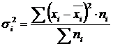
.

Medium of intragroup dispersions: .

There is a law connecting 3 types of dispersion. The total dispersion is equal to the sum of the average of intragroups and intergroup dispersion: .
This ratio is called rule of addition of dispersions.

An indicator is widely used in the analysis, which is a fraction of an intergroup dispersion in a common dispersion. He is called empirical determination coefficient (η 2): .
Square root from the empirical determination coefficient is called empirical correlation relationship (η):
.
It characterizes the effect of a feature laid in the base of the grouping, on the variation of an effective feature. The empirical correlation rate varies from 0 to 1.
We show its practical use on the following example (Table 1).

Example number 1. Table 1 - labor productivity of two groups of workers of one of the workshops of NPO "Cyclone"

Calculate general and group average and dispersion:

The initial data for calculating the middle of the intragroup and intergroup dispersion are presented in Table. 2.
table 2
Calculation and Δ 2 in two groups of workers.

Groups workers	The number of workers, people.	Middle, children / shift.	Dispersion
Past technical training	5	95	42,0
Not underway technical training	5	81	231,2
All workers	10	88	185,6

Calculate the indicators. Average of intragroup dispersions:
.
Intergroup dispersion

Total dispersion:
Thus, the empirical correlation ratio :.

Along with the variation of quantitative signs, the variation of high-quality signs can also be observed. Such a study of the variation is achieved by calculating the following types of dispersions:

Undergroup dispersion of the share is determined by the formula

Where n I. - The number of units in individual groups.
The share of the studied feature in the entire population, which is determined by the formula:
Three types of dispersion are related to each other:
.

This ratio of dispersions is called the theorem of the addition of dispersions of the trait share.

In many cases, it is necessary to introduce another one numerical characteristic To measure degree scatteringrandom ξ , around her mathematical expectation.

Definition. Dispersion random variable ξ called the number.

D ξ.= M (ξ-m ξ) 2 . (1)

In other words, the dispersion is expected value Square deviation of the values \u200b\u200bof a random variable from its average value.

called middle quadratic Deviation

values ξ .

If the dispersion characterizes the average deflection square ξ OT. Mξ., the number can be viewed as some average characteristic of the deviation itself, more precisely, the values \u200b\u200b| ξ-mξ. |.

The following two properties of the dispersion flow from the definition (1).

1. The dispersion of a constant value is zero. This fully corresponds to a visual meaning of dispersion as "scattering measures."

Indeed, if

ξ \u003d s that Mξ \u003d C. And, meaning Dξ \u003d m (C-C) 2 = M.0 = 0.

2. When multiplying a random variable ξ For a constant number with its dispersion is multiplied by C 2

D (Cξ.) = C. 2 Dξ. . (3)

Really

D (Cξ) \u003d M (C

= M (C. .

3. The following formula for calculating the dispersion is:

. (4)

Proof of this formula follows from the properties of mathematical expectation.

We have:

4. If values ξ 1 I. ξ 2 Independent, then the dispersion of their sum is equal to the sum of their dispersions:

Proof. To prove, use the properties of mathematical expectation. Let be Mξ. 1 \u003d M. 1 , Mξ. 2 \u003d M. 2, then.

Formula (5) is proved.

Since the dispersion of a random variable is by definition of the mathematical expectation of the magnitude ( ξ -m.) 2, where m \u003d mξ, That for calculating the dispersion, you can use the formulas obtained in §7 GL.II.

So, if ξ there is a DSV with the law of distribution

x. 1	x. 2	...
p. 1	p. 2	...

that will be:

. (7)

If a ξ continuous random variable distribution density p (X), then we get:

Dξ.= . (8)

If you use formula (4) to calculate the dispersion, you can get other formulas, namely:

, (9)

if the value ξ Discretal, I.

Dξ.= , (10)

if a ξ Distributed with density p.(x.).

Example 1. Let the value ξ Equally distributed on the segment [ a, B.]. Using formula (10) We get:

It can be shown that the dispersion of a random variable distributed by normal law with density

p (X)= , (11)

equal to σ 2.

Thus, it turns out the meaning of the parameter σ, which is included in the density expression (11) for the normal law; Σ. earth average quadratic deviation Values \u200b\u200bξ..

Example 2. Find a dispersion of random variable ξ divided by binomial law.

Decision . Taking advantage of the representation of ξ in the form

ξ = ξ 1 + ξ 2 + ξ n. (see example 2 §7 ch. II) and applying the formula of the addition of dispersions for independent values, we get

Dξ \u003d dξ. 1 + Dξ. 2 + Dξ n. .

Dispersion of any of the values ξ I. (i.= 1,2, n.) Count directly:

Dξ i \u003d \u200b\u200bm (ξ i) 2 - (Mξ I.) 2 \u003d 0 2 · q.+ 1 2 p.- p. 2 = p.(1-p.) = pQ..

Finally get

Dξ.= nPQ.where q \u003d1 - P..

The mathematical expectation (middle value) of the random value of X, given on a discrete probabilistic space, is called the number M \u003d M [x] \u003d σx i p i, if the series converges absolutely.

Appointment of service. Using the service online calculated mathematical expectation, dispersion and rms deviation (See example). In addition, a graph of the distribution function F (X) is built.

The properties of the mathematical expectation of a random variable

1. The mathematical expectation of a constant value is equal to her: M [C] \u003d C, C - constant;
2. M \u003d C M [x]
3. The mathematical expectation of the sum of random variables is equal to the sum of their mathematical expectations: m \u003d m [x] + m [y]
4. The mathematical expectation of the product of independent random variables is equal to the product of their mathematical expectations: m \u003d m [x] m [y], if x and y are independent.

Properties of dispersion

1. The dispersion of a constant value is zero: D (C) \u003d 0.
2. A permanent multiplier can be discarded from under the sign of the dispersion, erecting it into the square: D (k * x) \u003d k 2 d (x).
3. If the random variables x and y are independent, then the amount dispersion is equal to the amount of dispersions: D (x + y) \u003d d (x) + d (y).
4. If the random variables x and y are dependent: D (x + y) \u003d dx + dy + 2 (x-m [x]) (y-m [y])
5. Computational formula is valid for dispersion:
   D (x) \u003d m (x 2) - (m (x)) 2

Example. Known mathematical expectations and dispersion of two independent random variables x and y: m (x) \u003d 8, m (y) \u003d 7, d (x) \u003d 9, d (y) \u003d 6. Find mathematical expectation and dispersion Random variance Z \u003d 9x-8Y + 7.
Decision. Based on the properties of the mathematical expectation: M (z) \u003d m (9x-8y + 7) \u003d 9 * m (x) - 8 * m (y) + m (7) \u003d 9 * 8 - 8 * 7 + 7 \u003d 23 .
Based on the properties of the dispersion: D (z) \u003d d (9x-8Y + 7) \u003d D (9x) - D (8Y) + D (7) \u003d 9 ^ 2D (x) - 8 ^ 2D (y) + 0 \u003d 81 * 9 - 64 * 6 \u003d 345

Algorithm for calculating mathematical expectation

Properties of discrete random variables: all their values \u200b\u200bcan be renounced natural numbers; Each value to compare the probability other than zero.

1. Alternately multiply the pairs: X i per P i.
2. We fold the product of each pair x i p i.
   For example, for n \u003d 4: m \u003d σx i p i \u003d x 1 p 1 + x 2 p 2 + x 3 p 3 + x 4 p 4

Discrete Random Distribution Function Step, it increases with a jump at those points whose probabilities are positive.

Example number 1.

X I.	1	3	4	7	9
P I.	0.1	0.2	0.1	0.3	0.3

The mathematical expectation is found according to the formula m \u003d σx i p i.
Mathematical expectation M [x].
M [x] \u003d 1 * 0.1 + 3 * 0.2 + 4 * 0.1 + 7 * 0.3 + 9 * 0.3 \u003d 5.9
The dispersion is found according to the formula d \u003d σx 2 i p i - m [x] 2.
Dispersion D [x].
D [x] \u003d 1 2 * 0.1 + 3 2 * 0.2 + 4 2 * 0.1 + 7 2 * 0.3 + 9 2 * 0.3 - 5.9 2 \u003d 7.69
Average quadratic deviation σ (x).
Σ \u003d SQRT (D [x]) \u003d SQRT (7.69) \u003d 2.78

Example number 2. The discrete random value has the following range of distribution:

H.	-10	-5	0	5	10
r	but	0,32	2a.	0,41	0,03

Find the value A, mathematical expectation and the average quadratic deviation of this random variable.

Decision. The value of A find from the relation: Σp i \u003d 1
Σp i \u003d a + 0.32 + 2 A + 0.41 + 0.03 \u003d 0.76 + 3 a \u003d 1
0.76 + 3 a \u003d 1 or 0.24 \u003d 3 A, from where a \u003d 0.08

Example number 3. Determine the law of distribution of the discrete random variable, if its dispersion is known, and x 1 x 1 \u003d 6; x 2 \u003d 9; x 3 \u003d x; x 4 \u003d 15
p 1 \u003d 0.3; P 2 \u003d 0.3; p 3 \u003d 0.1; P 4 \u003d 0.3
d (x) \u003d 12.96

Decision.
Here it is necessary to make a formula for finding dispersion D (x):
d (x) \u003d x 1 2 p 1 + x 2 2 p 2 + x 3 2 p 3 + x 4 2 p 4 -m (x) 2
where Miethazza M (x) \u003d x 1 p 1 + x 2 P 2 + x 3 p 3 + x 4 P 4
For our data
m (x) \u003d 6 * 0,3 + 9 * 0,3 + x 3 * 0.1 + 15 * 0.3 \u003d 9 + 0.1x 3
12.96 \u003d 6 2 0.3 + 9 2 0.3 + x 3 2 0.1 + 15 2 0.3- (9 + 0.1x 3) 2
or -9/100 (x 2 -20x + 96) \u003d 0
Accordingly, it is necessary to find the roots of the equation, and there will be two.
x 3 \u003d 8, x 3 \u003d 12
Choose the one that satisfies the condition X 1 x 3 \u003d 12

Discrete random variable
x 1 \u003d 6; x 2 \u003d 9; x 3 \u003d 12; x 4 \u003d 15
p 1 \u003d 0.3; P 2 \u003d 0.3; p 3 \u003d 0.1; P 4 \u003d 0.3

The dispersion of a random variable is a measure of the scatter of the values \u200b\u200bof this value. Small dispersion means that the values \u200b\u200bare grouped close to each other. A large dispersion indicates a strong scattering of values. The concept of dispersion of a random variable is applied in statistics. For example, if you compare the dispersion of the values \u200b\u200bof two values \u200b\u200b(such as the results of observations of men's and female patients), you can check the significance of some variable. Also, the dispersion is used in constructing statistical models, since the small dispersion can be a sign that you excessively customize the values.

Steps

Calculation of sample dispersion

1. Write down the sample values. In most cases, only samples of certain general aggregates are available to statistics. For example, as a rule, statistics do not analyze the costs of the content of the totality of all cars in Russia - they analyze the random sample of several thousand cars. Such a sample will help determine the average expenses for the car, but most likely the value obtained will be far from real.

   • For example, we analyze the number of buns sold in a cafe for 6 days taken in random order. The sample has the following form: 17, 15, 23, 7, 9, 13. This is a sample, not a totality, because we have no data on bun sold for every day of the cafe.
   • If you are given a totality, and not a sample of values, go to the next section.

2. Record the formula to calculate the sample dispersion. The dispersion is a measure of scattering of certain values. The closer the value of the dispersion to zero, the closer the value is grouped together to each other. Working with a sample of values, use the following formula to calculate the dispersion:

   • S 2 (\\ DisplayStyle S ^ (2)) = ∑[( X i (\\ DisplayStyle X_ (I)) - X̅) 2 (\\ DisplayStyle ^ (2))] / (n - 1)
   • S 2 (\\ DisplayStyle S ^ (2)) - This is a dispersion. Dispersion is measured in square units of measurement.
   • X i (\\ DisplayStyle X_ (I)) - Each value in the sample.
   • X i (\\ DisplayStyle X_ (I)) It is necessary to subtract x̅, build a square, and then fold the results obtained.
   • x̅ - selective mean (average sample value).
   • n - the number of values \u200b\u200bin the sample.

3. Calculate the average sample value. It is indicated as X̅. The average sampling value is calculated as the usual arithmetic average: fold all the values \u200b\u200bin the sample, and then the result is divided by the number of values \u200b\u200bin the sample.

   • In our example, fold the values \u200b\u200bin the sample: 15 + 17 + 23 + 7 + 9 + 13 \u003d 84
     Now the result is divided by the number of values \u200b\u200bin the sample (in our example, they are 6): 84 ÷ 6 \u003d 14.
     Selective average x̅ \u003d 14.
   • Selective average is a central value around which values \u200b\u200bare distributed in the sample. If the values \u200b\u200bin the sample are grouped around the sample medium, then the dispersion is small; Otherwise, the dispersion is large.

4. Delete the selected average of each value in the sample. Now calculate the difference X i (\\ DisplayStyle X_ (I)) - X̅, where X i (\\ DisplayStyle X_ (I)) - Each value in the sample. Each result obtained testifies to the deviation of a particular value from the sample medium, that is, how far this value is from the average sample value.

   • In our example:
     X 1 (\\ DisplayStyle X_ (1)) - X̅ \u003d 17 - 14 \u003d 3
     x 2 (\\ displaystyle x_ (2)) - X̅ \u003d 15 - 14 \u003d 1
     x 3 (\\ DisplayStyle X_ (3)) - x̅ \u003d 23 - 14 \u003d 9
     x 4 (\\ DisplayStyle X_ (4)) - x̅ \u003d 7 - 14 \u003d -7
     x 5 (\\ displaystyle x_ (5)) - x̅ \u003d 9 - 14 \u003d -5
     X 6 (\\ DisplayStyle X_ (6)) - x̅ \u003d 13 - 14 \u003d -1
   • The correctness of the results obtained is easy to check, since their sum should be zero. This is due to the definition of the mean value, since negative values \u200b\u200b(distances from the average value to smaller values) are fully compensated by positive values \u200b\u200b(distances from the average value to large values).

5. As noted above, the amount of differences X i (\\ DisplayStyle X_ (I)) - X̅ must be zero. This means that the average dispersion is always equal to zero, which does not give any idea of \u200b\u200bscattering the values \u200b\u200bof a certain amount. To solve this problem, take each difference to the square X i (\\ DisplayStyle X_ (I)) - X̅. This will lead to the fact that you will only receive positive numbers that, when adding, never give 0.

   • In our example:
     ( X 1 (\\ DisplayStyle X_ (1)) - X̅) 2 \u003d 3 2 \u003d 9 (\\ displaystyle ^ (2) \u003d 3 ^ (2) \u003d 9)
     (x 2 (\\ displayStyle (X_ (2)) - X̅) 2 \u003d 1 2 \u003d 1 (\\ displayStyle ^ (2) \u003d 1 ^ (2) \u003d 1)
     9 2 = 81
     (-7) 2 = 49
     (-5) 2 = 25
     (-1) 2 = 1
   • You found a square of the difference - X̅) 2 (\\ DisplayStyle ^ (2)) For each value in the sample.

6. Calculate the sum of the squares of differences. That is, find the part of the formula that is written as follows: σ [( X i (\\ DisplayStyle X_ (I)) - X̅) 2 (\\ DisplayStyle ^ (2))]. Here the sign Σ means the sum of the squares of the differences for each value X i (\\ DisplayStyle X_ (I)) In the sample. You have already found squares of differences (X i (\\ DisplayStyle (X_ (I)) - X̅) 2 (\\ DisplayStyle ^ (2)) For each value X i (\\ DisplayStyle X_ (I)) in the sample; Now just fold these squares.

   • In our example: 9 + 1 + 81 + 49 + 25 + 1 \u003d 166 .

7. The resulting result is divided into n - 1, where n is the number of values \u200b\u200bin the sample. Some time ago, for calculating the dispersion of the statistics, the result was simply on n; In this case, you will receive the average size of the dispersion square, which is ideal for describing the dispersion of this sample. But remember that any sample is only a small part of the general set of values. If you take another sample and perform the same calculations, you will receive another result. As it turned out, dividing on N - 1 (and not just on N) gives a more accurate assessment of the dispersion of the general population, which you are interested in. The division on N - 1 became generally accepted, so it is included in the formula for calculating the sample dispersion.

   • In our example, the sample includes 6 values, that is, n \u003d 6.
     Sampling dispersion \u003d. S 2 \u003d 166 6 - 1 \u003d (\\ displaystyle s ^ (2) \u003d (\\ FRAC (166) (6-1)) \u003d) 33,2

8. Difference dispersion from standard deviation. Note that the formula is present in the formula, so the dispersion is measured in square units of measuring the analyzed value. Sometimes such a magnitude is quite difficult to operate; In such cases, use the standard deviation, which is equally square root from the dispersion. That is why the sample dispersion is indicated as S 2 (\\ DisplayStyle S ^ (2)), and the standard deviation of the sample - as S (\\ DisplayStyle S).

   • In our example, the standard deviation of the sample: S \u003d √33,2 \u003d 5.76.

   Calculation of dispersion of aggregate

   1. Analyze some totality of values. The aggregate includes all the values \u200b\u200bof the value under consideration. For example, if you are studying the age of residents of the Leningrad region, the aggregate includes the age of all residents of this area. In the case of working with a set, it is recommended to create a table and make a set of totality. Consider the following example:

      • There are 6 aquariums in some room. In each aquarium, the following number of fish lives:
        x 1 \u003d 5 (\\ displaystyle x_ (1) \u003d 5)
        x 2 \u003d 5 (\\ displaystyle x_ (2) \u003d 5)
        x 3 \u003d 8 (\\ displaystyle x_ (3) \u003d 8)
        x 4 \u003d 12 (\\ displaystyle x_ (4) \u003d 12)
        x 5 \u003d 15 (\\ displaystyle x_ (5) \u003d 15)
        x 6 \u003d 18 (\\ displaystyle x_ (6) \u003d 18)

   2. Write down the formula to calculate the dispersion of the general population. Since the combination includes all values \u200b\u200bof some value, the formula below allows you to obtain the exact value of the dispersion of the set. In order to distinguish the dispersion of a set of sampling dispersion (the value of which is only estimated), the statistics use different variables:

      • σ 2 (\\ DisplayStyle ^ (2)) = (∑( X i (\\ DisplayStyle X_ (I)) - μ) 2 (\\ DisplayStyle ^ (2))) / N.
      • σ 2 (\\ DisplayStyle ^ (2)) - Dispersion of the aggregate (read as "sigma in a square"). Dispersion is measured in square units of measurement.
      • X i (\\ DisplayStyle X_ (I)) - Each value in the aggregate.
      • Σ - Sign of the amount. That is, from each value X i (\\ DisplayStyle X_ (I)) It is necessary to subtract μ, build a square, and then fold the results obtained.
      • μ is the average set value.
      • n - the number of values \u200b\u200bin the general population.

   3. Calculate the mean value of the totality. When working with the general set, its average value is indicated as μ (MJ). The average set value is calculated as the usual average arithmetic: fold all the values \u200b\u200bin the general population, and then the result is divided by the number of values \u200b\u200bin the general set.

      • Keep in mind that the average values \u200b\u200bare not always calculated as the arithmetic average.
      • In our example, the mean value of the totality: μ \u003d 5 + 5 + 8 + 12 + 15 + 18 6 (\\ displayStyle (\\ FRAC (5 + 5 + 8 + 12 + 15 + 18) (6))) = 10,5

   4. Delete the average set value from each value in the general population. The closer the value of the difference to zero, the closer the specific value to the average value of the totality. Find the difference between each value in the aggregate and its average value, and you will receive the first idea of \u200b\u200bthe distribution of values.

      • In our example:
        X 1 (\\ DisplayStyle X_ (1)) - μ \u003d 5 - 10.5 \u003d -5.5
        x 2 (\\ displaystyle x_ (2)) - μ \u003d 5 - 10.5 \u003d -5.5
        x 3 (\\ DisplayStyle X_ (3)) - μ \u003d 8 - 10.5 \u003d -2.5
        x 4 (\\ DisplayStyle X_ (4)) - μ \u003d 12 - 10.5 \u003d 1.5
        x 5 (\\ displaystyle x_ (5)) - μ \u003d 15 - 10.5 \u003d 4.5
        X 6 (\\ DisplayStyle X_ (6)) - μ \u003d 18 - 10.5 \u003d 7.5

   5. Earb the square each result. The difference values \u200b\u200bwill be both positive and negative; If you apply these values \u200b\u200bto the numeric straight, then they will lie on the right and to the left of the average value of the set. This is not suitable for calculating the dispersion, since positive and negative numbers compensate each other. Therefore, take a square each difference in order to get exceptionally positive numbers.

      • In our example:
        ( X i (\\ DisplayStyle X_ (I)) - μ) 2 (\\ DisplayStyle ^ (2)) For each value of the set (from i \u003d 1 to i \u003d 6):
        (-5,5) 2 (\\ DisplayStyle ^ (2)) = 30,25
        (-5,5) 2 (\\ DisplayStyle ^ (2))where x n (\\ displaystyle x_ (n)) - Last value in the general population.
      • To calculate the average value of the results, you need to find their sum and divide it on n: (( X 1 (\\ DisplayStyle X_ (1)) - μ) 2 (\\ DisplayStyle ^ (2)) + ( x 2 (\\ displaystyle x_ (2)) - μ) 2 (\\ DisplayStyle ^ (2)) + ... + ( x n (\\ displaystyle x_ (n)) - μ) 2 (\\ DisplayStyle ^ (2))) / N.
      • Now write down the explanation using variables: (σ ( X i (\\ DisplayStyle X_ (I)) - μ) 2 (\\ DisplayStyle ^ (2))) / n and we obtain a formula for calculating the dispersion of the totality.