Power series expansion in powers of x. Expansion of functions into power series

If the function f(x) has on some interval containing a point a, derivatives of all orders, then the Taylor formula can be applied to it:

where rn- the so-called residual term or the remainder of the series, it can be estimated using the Lagrange formula:

, where the number x is enclosed between X and a.

If for some value x r n®0 at n®¥, then in the limit the Taylor formula for this value turns into a convergent formula Taylor series:

So the function f(x) can be expanded into a Taylor series at the considered point X, if:

1) it has derivatives of all orders;

2) the constructed series converges at this point.

At a=0 we get a series called near Maclaurin:

Example 1 f(x)= 2x.

Solution. Let us find the values ​​of the function and its derivatives at X=0

f(x) = 2x, f( 0) = 2 0 =1;

f¢(x) = 2x ln2, f¢( 0) = 2 0 ln2=ln2;

f¢¢(x) = 2x ln 2 2, f¢¢( 0) = 2 0 log 2 2= log 2 2;

f(n)(x) = 2x ln n 2, f(n)( 0) = 2 0 ln n 2=ln n 2.

Substituting the obtained values ​​of the derivatives into the Taylor series formula, we get:

The radius of convergence of this series is equal to infinity, so this expansion is valid for -¥<x<+¥.

Example 2 X+4) for the function f(x)= e x.

Solution. Finding the derivatives of the function e x and their values ​​at the point X=-4.

f(x)= e x, f(-4) = e -4 ;

f¢(x)= e x, f¢(-4) = e -4 ;

f¢¢(x)= e x, f¢¢(-4) = e -4 ;

f(n)(x)= e x, f(n)( -4) = e -4 .

Therefore, the desired Taylor series of the function has the form:

This decomposition is also valid for -¥<x<+¥.

Example 3 . Expand function f(x)=ln x in a series by degrees ( X- 1),

(i.e. in a Taylor series in the vicinity of the point X=1).

Solution. We find the derivatives of this function.

Substituting these values ​​into the formula, we obtain the desired Taylor series:

With the help of d'Alembert's test, one can verify that the series converges when

½ X- 1½<1. Действительно,

The series converges if ½ X- 1½<1, т.е. при 0<x<2. При X=2 we obtain an alternating series that satisfies the conditions of the Leibniz test. At X=0 function is not defined. Thus, the region of convergence of the Taylor series is the half-open interval (0;2].

Let us present the expansions obtained in this way in the Maclaurin series (i.e., in a neighborhood of the point X=0) for some elementary functions:

(2) ,

(3) ,

( the last expansion is called binomial series)

Example 4 . Expand the function into a power series

Solution. In decomposition (1), we replace X on the - X 2 , we get:

Example 5 . Expand the function in a Maclaurin series

Solution. We have

Using formula (4), we can write:

substituting instead of X into the formula -X, we get:

From here we find:

Expanding the brackets, rearranging the terms of the series and making a reduction of similar terms, we get

This series converges in the interval

(-1;1) since it is derived from two series, each of which converges in this interval.

Comment .

Formulas (1)-(5) can also be used to expand the corresponding functions in a Taylor series, i.e. for the expansion of functions in positive integer powers ( Ha). To do this, it is necessary to perform such identical transformations on a given function in order to obtain one of the functions (1) - (5), in which instead of X costs k( Ha) m , where k is a constant number, m is a positive integer. It is often convenient to change the variable t=Ha and expand the resulting function with respect to t in the Maclaurin series.

This method illustrates the theorem on the uniqueness of the expansion of a function in a power series. The essence of this theorem is that in the neighborhood of the same point, two different power series cannot be obtained that would converge to the same function, no matter how its expansion is performed.

Example 6 . Expand the function in a Taylor series in a neighborhood of a point X=3.

Solution. This problem can be solved, as before, using the definition of the Taylor series, for which it is necessary to find the derivatives of the functions and their values ​​at X=3. However, it will be easier to use the existing decomposition (5):

The resulting series converges at or -3<x- 3<3, 0<x< 6 и является искомым рядом Тейлора для данной функции.

Example 7 . Write a Taylor series in powers ( X-1) features .

Solution.

The series converges at , or 2< x£5.

Students of higher mathematics should be aware that the sum of a certain power series belonging to the interval of convergence of the series given to us turns out to be a continuous and unlimited number of times differentiated function. The question arises: is it possible to assert that a given arbitrary function f(x) is the sum of some power series? That is, under what conditions can the function f(x) be represented by a power series? The importance of this question lies in the fact that it is possible to approximately replace the function f(x) by the sum of the first few terms of the power series, that is, by a polynomial. Such a replacement of a function by a rather simple expression - a polynomial - is also convenient when solving some problems, namely: when solving integrals, when calculating, etc.

It is proved that for some function f(x), in which derivatives up to the (n + 1)th order, including the last one, can be calculated, in the neighborhood (α - R; x 0 + R) of some point x = α formula:

This formula is named after the famous scientist Brook Taylor. The series that is obtained from the previous one is called the Maclaurin series:

The rule that makes it possible to expand in a Maclaurin series:

1. Determine the derivatives of the first, second, third ... orders.
2. Calculate what the derivatives at x=0 are.
3. Write the Maclaurin series for this function, and then determine the interval of its convergence.
4. Determine the interval (-R;R), where the remainder of the Maclaurin formula

R n (x) -> 0 for n -> infinity. If one exists, the function f(x) in it must coincide with the sum of the Maclaurin series.

Consider now the Maclaurin series for individual functions.

1. So, the first will be f(x) = e x. Of course, according to its features, such a function has derivatives of very different orders, and f (k) (x) \u003d e x, where k equals everything Let us substitute x \u003d 0. We get f (k) (0) \u003d e 0 \u003d 1, k \u003d 1.2 ... Based on the foregoing, the series e x will look like this:

2. The Maclaurin series for the function f(x) = sin x. Immediately clarify that the function for all unknowns will have derivatives, besides f "(x) \u003d cos x \u003d sin (x + n / 2), f "" (x) \u003d -sin x \u003d sin (x +2*n/2)..., f(k)(x)=sin(x+k*n/2), where k is equal to any natural number.That is, by making simple calculations, we can conclude that the series for f(x) = sin x will look like this:

3. Now let's try to consider the function f(x) = cos x. It has derivatives of arbitrary order for all unknowns, and |f (k) (x)| = |cos(x+k*n/2)|<=1, k=1,2... Снова-таки, произведя определенные расчеты, получим, что ряд для f(х) = cos х будет выглядеть так:

So, we have listed the most important functions that can be expanded in the Maclaurin series, but they are supplemented by Taylor series for some functions. Now we will list them. It is also worth noting that Taylor and Maclaurin series are an important part of the practice of solving series in higher mathematics. So, Taylor series.

1. The first will be a row for f-ii f (x) = ln (1 + x). As in the previous examples, given us f (x) = ln (1 + x), we can add a series using the general form of the Maclaurin series. however, for this function, the Maclaurin series can be obtained much more simply. After integrating a certain geometric series, we get a series for f (x) = ln (1 + x) of such a sample:

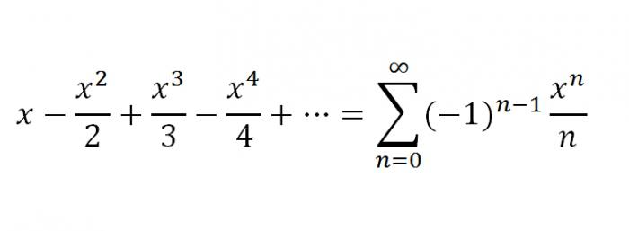
2. And the second, which will be final in our article, will be a series for f (x) \u003d arctg x. For x belonging to the interval [-1; 1], the expansion is valid:

That's all. In this article, the most used Taylor and Maclaurin series in higher mathematics, in particular, in economic and technical universities, were considered.

"Find the Maclaurin expansion of f(x)"- this is exactly what the task in higher mathematics sounds like, which some students can do, while others cannot cope with examples. There are several ways to expand a series in powers, here we will give a method for expanding functions in a Maclaurin series. When developing a function in a series, you need to be good at calculating derivatives.

Example 4.7 Expand a function into a series in powers of x

Calculations: We perform the expansion of the function according to the Maclaurin formula. First, we expand the denominator of the function into a series

Finally, we multiply the expansion by the numerator.
The first term is the value of the function at zero f (0) = 1/3.
Find the derivatives of the first and higher order functions f (x) and the value of these derivatives at the point x=0




Further, with the pattern of changing the value of derivatives to 0, we write the formula for the n-th derivative

So, we represent the denominator as an expansion in the Maclaurin series

We multiply by the numerator and get the desired expansion of the function in a series in powers of x

As you can see, there is nothing complicated here.
All key points are based on the ability to calculate derivatives and quickly generalize the value of the derivative of higher orders at zero. The following examples will help you learn how to quickly expand a function into a series.

Example 4.10 Find the Maclaurin expansion of a function

Calculations: As you may have guessed, we will expand the cosine in the numerator in a series. To do this, you can use formulas for infinitesimal values, or you can derive the cosine expansion in terms of derivatives. As a result, we arrive at the next series in powers of x

As you can see, we have a minimum of calculations and a compact representation of the series expansion.

Example 4.16 Expand a function into a series in powers of x:
7/(12-x-x^2)
Calculations: In this kind of examples, it is necessary to expand the fraction through the sum of simple fractions.
How to do this, we will not show now, but with the help of indefinite coefficients we will arrive at the sum of ex fractions.
Next, we write the denominators in exponential form

It remains to expand the terms using the Maclaurin formula. Summing up the terms with the same powers of "x", we compose the formula for the general term of the expansion of the function in a series



The last part of the transition to the series at the beginning is difficult to implement, since it is difficult to combine the formulas for paired and unpaired indices (powers), but with practice you will get better at this.

Example 4.18 Find the Maclaurin expansion of a function

Calculations: Find the derivative of this function:

We expand the function into a series using one of the McLaren formulas:

We summarize the series term by term on the basis that both are absolutely coinciding. By integrating the entire series term by term, we obtain the expansion of the function into a series in powers of x

Between the last two lines of decomposition there is a transition which at the beginning will take you a lot of time. Generalizing a series formula is not easy for everyone, so don't worry about not being able to get a nice and compact formula.

Example 4.28 Find the Maclaurin expansion of the function:

We write the logarithm as follows

Using the Maclaurin formula, we expand the logarithm of the function in a series in powers of x

The final folding is at first glance complicated, but when alternating characters, you will always get something similar. Introductory lesson on the topic of function scheduling in a row is completed. Other no less interesting decomposition schemes will be discussed in detail in the following materials.

In the theory of functional series, the section devoted to the expansion of a function into a series occupies a central place.

Thus, the problem is posed: for a given function it is required to find such a power series

which converged on some interval and its sum was equal to
, those.

= ..

This task is called the problem of expanding a function into a power series.

A necessary condition for the expansion of a function into a power series is its differentiability an infinite number of times - this follows from the properties of convergent power series. This condition is satisfied, as a rule, for elementary functions in their domain of definition.

So let's assume that the function
has derivatives of any order. Can it be expanded into a power series, if so, how to find this series? The second part of the problem is easier to solve, so let's start with it.

Let's assume that the function
can be represented as the sum of a power series converging in an interval containing a point X 0 :

= .. (*)

where a 0 ,a 1 ,a 2 ,...,a P ,... – uncertain (yet) coefficients.

Let us put in equality (*) the value x = x 0 , then we get

.

We differentiate the power series (*) term by term

= ..

and putting here x = x 0 , we get

.

With the next differentiation, we get the series

= ..

assuming x = x 0 , we get
, where
.

After P-fold differentiation we get

Assuming in the last equality x = x 0 , we get
, where

So the coefficients are found

,
,
, …,
,….,

substituting which into a row (*), we get

The resulting series is called near taylor for function
.

Thus, we have established that if the function can be expanded into a power series in powers (x - x 0 ), then this expansion is unique and the resulting series is necessarily a Taylor series.

Note that the Taylor series can be obtained for any function that has derivatives of any order at the point x = x 0 . But this does not yet mean that an equal sign can be put between the function and the resulting series, i.e. that the sum of the series is equal to the original function. Firstly, such an equality can only make sense in the region of convergence, and the Taylor series obtained for the function may diverge, and secondly, if the Taylor series converges, then its sum may not coincide with the original function.

3.2. Sufficient conditions for the expansion of a function into a Taylor series

Let us formulate a statement with the help of which the stated problem will be solved.

If the function
in some neighborhood of the point x 0 has derivatives up to (n+ 1)-th order inclusive, then in this neighborhood we haveformula Taylor

whereR n (X)-residual term of the Taylor formula - has the form (Lagrange form)

where dotξ lies between x and x 0 .

Note that there is a difference between the Taylor series and the Taylor formula: the Taylor formula is a finite sum, i.e. P - fixed number.

Recall that the sum of the series S(x) can be defined as the limit of the functional sequence of partial sums S P (x) at some interval X:

.

According to this, to expand a function into a Taylor series means to find a series such that for any XX

We write the Taylor formula in the form where

notice, that
defines the error we get, replace the function f(x) polynomial S n (x).

If
, then
,those. the function expands into a Taylor series. Conversely, if
, then
.

Thus, we have proved criterion for the expansion of a function into a Taylor series.

In order that in some interval the functionf(x) expands in a Taylor series, it is necessary and sufficient that on this interval
, whereR n (x) is the remainder of the Taylor series.

With the help of the formulated criterion, one can obtain sufficientconditions for the expansion of a function into a Taylor series.

If insome neighborhood of the point x 0 the absolute values ​​of all derivatives of a function are limited by the same number M≥ 0, i.e.

, To in this neighborhood, the function expands into a Taylor series.

From the above it follows algorithmfunction expansion f(x) in a Taylor series in the vicinity of the point X 0 :

1. Finding derivative functions f(x):

f(x), f’(x), f”(x), f’”(x), f (n) (x),…

2. We calculate the value of the function and the values ​​of its derivatives at the point X 0

f(x 0 ), f'(x 0 ), f”(x 0 ), f’”(x 0 ), f (n) (x 0 ),…

3. We formally write the Taylor series and find the region of convergence of the resulting power series.

4. We check the fulfillment of sufficient conditions, i.e. establish for which X from the convergence region, remainder term R n (x) tends to zero at
or
.

The expansion of functions in a Taylor series according to this algorithm is called expansion of a function in a Taylor series by definition or direct decomposition.

16.1. Expansion of elementary functions in Taylor series and

Maclaurin

Let us show that if an arbitrary function is defined on the set
, in the vicinity of the point
has many derivatives and is the sum of a power series:

then you can find the coefficients of this series.

Substitute in a power series
. Then
.

Find the first derivative of the function
:

At
:
.

For the second derivative we get:

At
:
.

Continuing this procedure n once we get:
.

Thus, we got a power series of the form:

,

which is called near taylor for function
around the point
.

A special case of the Taylor series is Maclaurin series at
:

The remainder of the Taylor (Maclaurin) series is obtained by discarding the main series n the first terms and is denoted as
. Then the function
can be written as a sum n the first members of the series
and the remainder
:,

.

The rest is usually
expressed in different formulas.

One of them is in the Lagrange form:

, where
.
.

Note that in practice the Maclaurin series is used more often. Thus, in order to write the function
in the form of a sum of a power series, it is necessary:

1) find the coefficients of the Maclaurin (Taylor) series;

2) find the region of convergence of the resulting power series;

3) prove that the given series converges to the function
.

Theorem1 (a necessary and sufficient condition for the convergence of the Maclaurin series). Let the convergence radius of the series
. In order for this series to converge in the interval
to function
, it is necessary and sufficient that the following condition is satisfied:
within the specified interval.

Theorem 2. If derivatives of any order of a function
in some interval
limited in absolute value to the same number M, that is
, then in this interval the function
can be expanded in a Maclaurin series.

Example1 . Expand in a Taylor series around the point
function.

Solution.

.

,;

,
;

,
;

,

.......................................................................................................................................

,
;

Convergence area
.

Example2 . Expand function in a Taylor series around a point
.

Solution:

We find the value of the function and its derivatives at
.

,
;

,
;

...........……………………………

,
.

Substitute these values ​​in a row. We get:

or
.

Let us find the region of convergence of this series. According to the d'Alembert test, the series converges if

.

Therefore, for any this limit is less than 1, and therefore the area of ​​convergence of the series will be:
.

Let us consider several examples of the expansion into the Maclaurin series of basic elementary functions. Recall that the Maclaurin series:

.

converges on the interval
to function
.

Note that to expand the function into a series, it is necessary:

a) find the coefficients of the Maclaurin series for a given function;

b) calculate the radius of convergence for the resulting series;

c) prove that the resulting series converges to the function
.

Example 3 Consider the function
.

Solution.

Let us calculate the value of the function and its derivatives for
.

Then the numerical coefficients of the series have the form:

for anyone n. We substitute the found coefficients in the Maclaurin series and get:

Find the radius of convergence of the resulting series, namely:

.

Therefore, the series converges on the interval
.

This series converges to the function for any values , because on any interval
function and its absolute value derivatives are limited by the number .

Example4 . Consider the function
.

Solution.

:

It is easy to see that even-order derivatives
, and derivatives of odd order. We substitute the found coefficients in the Maclaurin series and get the expansion:

Let us find the interval of convergence of this series. According to d'Alembert:

for anyone . Therefore, the series converges on the interval
.

This series converges to the function
, because all its derivatives are limited to one.

Example5 .
.

Solution.

Let us find the value of the function and its derivatives at
:

Thus, the coefficients of this series:
and
, hence:

Similarly with the previous series, the area of ​​convergence
. The series converges to the function
, because all its derivatives are limited to one.

Note that the function
odd and series expansion in odd powers, function
– even and expansion in a series in even powers.

Example6 . Binomial series:
.

Solution.

Let us find the value of the function and its derivatives at
:

This shows that:

We substitute these values ​​of the coefficients in the Maclaurin series and obtain the expansion of this function in a power series:

Let's find the radius of convergence of this series:

Therefore, the series converges on the interval
. At the limit points at
and
series may or may not converge depending on the exponent
.

The studied series converges on the interval
to function
, that is, the sum of the series
at
.

Example7 . Let us expand the function in a Maclaurin series
.

Solution.

To expand this function into a series, we use the binomial series for
. We get:

Based on the property of power series (a power series can be integrated in the region of its convergence), we find the integral of the left and right parts of this series:

Find the area of ​​convergence of this series:
,

that is, the convergence region of this series is the interval
. Let us determine the convergence of the series at the ends of the interval. At

. This series is a harmonic series, that is, it diverges. At
we get a number series with a common term
.

The Leibniz series converges. Thus, the region of convergence of this series is the interval
.

16.2. Application of power series of powers in approximate calculations

Power series play an extremely important role in approximate calculations. With their help, tables of trigonometric functions, tables of logarithms, tables of values ​​of other functions that are used in various fields of knowledge, for example, in probability theory and mathematical statistics, were compiled. In addition, the expansion of functions in a power series is useful for their theoretical study. The main issue when using power series in approximate calculations is the question of estimating the error when replacing the sum of a series by the sum of its first n members.

Consider two cases:

the function is expanded into an alternating series;

the function is expanded into a constant-sign series.

Calculation using alternating series

Let the function
expanded into an alternating power series. Then, when calculating this function for a specific value we get a number series to which we can apply the Leibniz test. In accordance with this criterion, if the sum of a series is replaced by the sum of its first n members, then the absolute error does not exceed the first term of the remainder of this series, that is:
.

Example8 . Calculate
with an accuracy of 0.0001.

Solution.

We will use the Maclaurin series for
, substituting the value of the angle in radians:

If we compare the first and second members of the series with a given accuracy, then: .

Third expansion term:

less than the specified calculation accuracy. Therefore, to calculate
it suffices to leave two terms of the series, i.e.

.

In this way
.

Example9 . Calculate
with an accuracy of 0.001.

Solution.

We will use the binomial series formula. For this we write
as:
.

In this expression
,

Let's compare each of the terms of the series with the accuracy that is given. It's clear that
. Therefore, to calculate
it suffices to leave three members of the series.

or
.

Calculation using sign-positive series

Example10 . Calculate number with an accuracy of 0.001.

Solution.

In a row for a function
substitute
. We get:

Let us estimate the error that arises when the sum of the series is replaced by the sum of the first members. Let's write down the obvious inequality:

i.e. 2<<3. Используем формулу остаточного члена ряда в форме Лагранжа:
,
.

According to the condition of the problem, you need to find n such that the following inequality holds:
or
.

It is easy to check that when n= 6:
.

Hence,
.

Example11 . Calculate
with an accuracy of 0.0001.

Solution.

Note that to calculate the logarithms, one could apply the series for the function
, but this series converges very slowly and 9999 terms would have to be taken to achieve the given accuracy! Therefore, to calculate logarithms, as a rule, a series for the function is used
, which converges on the interval
.

Compute
with this row. Let
, then .

Hence,
,

In order to calculate
with a given accuracy, take the sum of the first four terms:
.

The rest of the row
discard. Let's estimate the error. It's obvious that

or
.

Thus, in the series that was used for the calculation, it was enough to take only the first four terms instead of 9999 in the series for the function
.

Questions for self-diagnosis

1. What is a Taylor series?

2. what kind of series did Maclaurin have?

3. Formulate a theorem on the expansion of a function in a Taylor series.

4. Write the expansion in the Maclaurin series of the main functions.

5. Indicate the areas of convergence of the considered series.

6. How to estimate the error in approximate calculations using power series?