How to find the variance of a series. Calculation of group, intergroup and total variance (according to the rule of addition of variances)
If the population is divided into groups according to the studied attribute, then the following types of dispersion can be calculated for this population: general, group (intragroup), average from group (average from within group), intergroup.
Initially, it calculates the coefficient of determination, which shows how much of the total variation of the studied trait is the intergroup variation, i.e. due to the grouping attribute:
The empirical correlation ratio characterizes the tightness of the connection between the grouping (factor) and the effective ones.
The empirical correlation ratio can take values from 0 to 1.
To assess the tightness of the relationship based on the empirical correlation ratio, you can use the Chaddock ratios:
Example 4. There is the following data on the performance of work by design and survey organizations different shapes property:
Define:
1) total variance;
2) group variances;
3) the average of the group variances;
4) intergroup variance;
5) total variance based on the variance addition rule;
6) the coefficient of determination and the empirical correlation ratio.
Draw conclusions.
Solution:
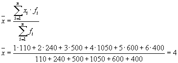
1. Let us determine the average volume of work performed by enterprises of two forms of ownership:
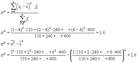
Let's calculate the total variance:
![]()
2. Let's define the group means:
![]() million rubles;
million rubles;
![]() RUB million
RUB million
Group variances:
![]() ;
;
3. Let's calculate the average of the group variances:
4. Determine the intergroup variance:
5. Let's calculate the total variance based on the variance addition rule:
6. Let's define the coefficient of determination:
![]() .
.
Thus, the amount of work performed by design and survey organizations by 22% depends on the form of ownership of enterprises.
The empirical correlation ratio is calculated by the formula
![]() .
.
The value of the calculated indicator indicates that the dependence of the volume of work on the form of ownership of the enterprise is not large.
Example 5. As a result of a survey of the technological discipline of production sites, the following data were obtained:
Determine the coefficient of determination
Along with the study of the variation of a trait across the entire population as a whole, it is often necessary to trace quantitative changes signs by groups into which the totality is divided, as well as between groups. This study of variation is achieved through calculation and analysis. different types variance.
Allocate general, intergroup and intragroup variance.
Total variance σ 2 measures the variation of a trait across the entire population under the influence of all factors that caused this variation,.
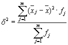
Intergroup variance(δ) characterizes systematic variation, i.e. differences in the size of the trait under study arising under the influence of the trait-factor underlying the grouping. It is calculated by the formula:  .
.
Intra-group variance (σ) reflects random variation, i.e. a part of the variation that occurs under the influence of unaccounted factors and does not depend on the attribute-factor underlying the grouping. It is calculated by the formula:  .
.
Average of within-group variances:  .
.
There is a law linking 3 types of dispersion. The total variance is equal to the sum of the average of intragroup and intergroup variances: ![]() .
.
This ratio is called variance addition rule.
The analysis widely uses an indicator that represents the proportion of intergroup variance in total variance... It bears the name empirical coefficient of determination (η 2): .
The square root of the empirical coefficient of determination is called empirical correlation ratio (η):
 .
.
It characterizes the influence of the trait underlying the grouping on the variation of the effective trait. The empirical correlation ratio ranges from 0 to 1.
Let's show its practical use on the following example (Table 1).
Example # 1. Table 1 - Labor productivity of two groups of workers of one of the workshops of NPO "Cyclone"
Let's calculate the total and group averages and variances:
The initial data for calculating the average of intragroup and intergroup variance are presented in table. 2.
table 2
Calculation and δ 2 for two groups of workers.
|
Worker groups | Number of workers, people | Average, children / shift | Dispersion |
| Passed technical training | 5 | 95 | 42,0 |
| Those who have not completed technical training | 5 | 81 | 231,2 |
| All workers | 10 | 88 | 185,6 |
 .
.
Intergroup variance
Total variance:
Thus, the empirical correlation is:.
Along with the variation in quantitative traits, variation in qualitative traits can also be observed. This study of variation is achieved by calculating the following types of variances:
Intra-group variance of the share is determined by the formula
where n i- the number of units in separate groups.The share of the trait under study in the entire population, which is determined by the formula:
The three types of variance are related as follows:
This ratio of variances is called the theorem of addition of variances of the share of a feature.
Dispersion random variable is a measure of the spread in the values of this quantity. Low variance means that the values are grouped close to each other. Large variance indicates a strong scatter of values. The concept of variance of a random variable is used in statistics. For example, if you compare the variance of the values of two variables (such as observations of male and female patients), you can test the significance of a variable. Variance is also used when building statistical models, as low variance can be an indication that you are overfitting the values.Steps
Calculating Sample Variance
-
Write down the sample values. In most cases, only samples of certain populations are available to statisticians. For example, as a rule, statisticians do not analyze the costs of maintaining the aggregate of all cars in Russia - they analyze a random sample of several thousand cars. Such a sample will help determine the average cost of a car, but, most likely, the resulting value will be far from the real one.
- For example, let's analyze the number of buns sold in a cafe in 6 days, taken in random order. The sample looks like this: 17, 15, 23, 7, 9, 13. This is a sample, not a population, because we do not have data on the sold buns for each day the cafe is open.
- If you are given a population rather than a sample of values, skip to the next section.
-
Write down the formula to calculate the sample variance. Dispersion is a measure of the spread of values of a certain quantity. How closer meaning variance to zero, the closer the values are grouped to each other. When working with a sample of values, use the following formula to calculate the variance:
- s 2 (\ displaystyle s ^ (2)) = ∑[(x i (\ displaystyle x_ (i))- x̅) 2 (\ displaystyle ^ (2))] / (n - 1)
- s 2 (\ displaystyle s ^ (2)) Is the variance. Dispersion is measured in square units measurements.
- x i (\ displaystyle x_ (i))- each value in the sample.
- x i (\ displaystyle x_ (i)) subtract x̅, square it, and then add the results.
- x̅ - sample mean (sample mean).
- n is the number of values in the sample.
-
Calculate the average of the sample. It is denoted as x̅. The sample mean is calculated as a normal arithmetic mean: add up all the values in the sample, and then divide the result by the number of values in the sample.
- In our example, add the values in the sample: 15 + 17 + 23 + 7 + 9 + 13 = 84
Now divide the result by the number of values in the sample (in our example there are 6 of them): 84 ÷ 6 = 14.
Sample mean x̅ = 14. - The sample mean is the central value around which the values in the sample are distributed. If the values in the sample are grouped around the sample mean, then the variance is small; otherwise, the variance is large.
- In our example, add the values in the sample: 15 + 17 + 23 + 7 + 9 + 13 = 84
-
Subtract the sample mean from each value in the sample. Now calculate the difference x i (\ displaystyle x_ (i))- x̅, where x i (\ displaystyle x_ (i))- each value in the sample. Each result obtained indicates the degree of deviation of a particular value from the sample mean, that is, how far this value is from the sample mean.
- In our example:
x 1 (\ displaystyle x_ (1))- x̅ = 17 - 14 = 3
x 2 (\ displaystyle x_ (2))- x̅ = 15 - 14 = 1
x 3 (\ displaystyle x_ (3))- x̅ = 23 - 14 = 9
x 4 (\ displaystyle x_ (4))- x̅ = 7 - 14 = -7
x 5 (\ displaystyle x_ (5))- x̅ = 9 - 14 = -5
x 6 (\ displaystyle x_ (6))- x̅ = 13 - 14 = -1 - The correctness of the results obtained is easy to verify, since their sum should be equal to zero. This is due to the determination of the mean, since negative values (distances from the mean to lower values) are completely compensated by positive values (distances from the mean to larger values).
- In our example:
-
As noted above, the sum of the differences x i (\ displaystyle x_ (i))- x̅ must be zero. It means that mean variance is always zero, which does not give any idea about the spread of values of some quantity. To solve this problem, square each difference x i (\ displaystyle x_ (i))- x̅. This will result in you only getting positive numbers which never add up to 0.
- In our example:
(x 1 (\ displaystyle x_ (1))- x̅) 2 = 3 2 = 9 (\ displaystyle ^ (2) = 3 ^ (2) = 9)
(x 2 (\ displaystyle (x_ (2))- x̅) 2 = 1 2 = 1 (\ displaystyle ^ (2) = 1 ^ (2) = 1)
9 2 = 81
(-7) 2 = 49
(-5) 2 = 25
(-1) 2 = 1 - You found the squared difference - x̅) 2 (\ displaystyle ^ (2)) for each value in the sample.
- In our example:
-
Calculate the sum of the squares of the differences. That is, find the part of the formula that is written like this: ∑ [( x i (\ displaystyle x_ (i))- x̅) 2 (\ displaystyle ^ (2))]. Here the sign Σ means the sum of the squares of the differences for each value x i (\ displaystyle x_ (i)) in the sample. You have already found the squares of the differences (x i (\ displaystyle (x_ (i))- x̅) 2 (\ displaystyle ^ (2)) for each value x i (\ displaystyle x_ (i)) in the sample; now just add those squares.
- In our example: 9 + 1 + 81 + 49 + 25 + 1 = 166 .
-
Divide the result by n - 1, where n is the number of values in the sample. Some time ago, to calculate the variance of a sample, statistics simply divided the result by n; in this case, you will get the mean squared variance, which is ideal for describing the variance of a given sample. But remember that any sample is only a small part of the the general population values. If you take a different sample and do the same calculations, you get a different result. As it turns out, dividing by n - 1 (rather than just n) gives a more accurate estimate of the population variance, which is what you are interested in. Division by n - 1 has become common, so it is included in the formula for calculating sample variance.
- In our example, the sample includes 6 values, that is, n = 6.
Sample variance = s 2 = 166 6 - 1 = (\ displaystyle s ^ (2) = (\ frac (166) (6-1)) =) 33,2
- In our example, the sample includes 6 values, that is, n = 6.
-
The difference between variance and standard deviation. Note that there is an exponent in the formula, so variance is measured in square units of the analyzed quantity. Sometimes it is quite difficult to operate with such a value; in such cases, the standard deviation is used, which is equal to square root from variance. That is why the sample variance is denoted as s 2 (\ displaystyle s ^ (2)), a standard deviation sampling - how s (\ displaystyle s).
- In our example, the sample standard deviation is s = √33.2 = 5.76.
Calculating the variance of a population
-
Analyze a set of values. The set includes all values of the considered quantity. For example, if you are studying the age of residents Leningrad region, then the totality includes the age of all residents of this area. If you are working with a population, it is recommended that you create a table and enter the population values into it. Consider the following example:
- In some room there are 6 aquariums. Each aquarium has the following number of fish:
x 1 = 5 (\ displaystyle x_ (1) = 5)
x 2 = 5 (\ displaystyle x_ (2) = 5)
x 3 = 8 (\ displaystyle x_ (3) = 8)
x 4 = 12 (\ displaystyle x_ (4) = 12)
x 5 = 15 (\ displaystyle x_ (5) = 15)
x 6 = 18 (\ displaystyle x_ (6) = 18)
- In some room there are 6 aquariums. Each aquarium has the following number of fish:
-
Write down the formula for calculating the variance of the population. Since the aggregate includes all values of a certain quantity, the formula below allows one to obtain exact value variance of the population. In order to distinguish the variance of the population from the variance of the sample (the value of which is only an estimate), statisticians use various variables:
- σ 2 (\ displaystyle ^ (2)) = (∑(x i (\ displaystyle x_ (i)) - μ) 2 (\ displaystyle ^ (2))) / n
- σ 2 (\ displaystyle ^ (2))- variance of the population (read as "sigma squared"). Dispersion is measured in square units.
- x i (\ displaystyle x_ (i))- each value in aggregate.
- Σ is the sum sign. That is, from each value x i (\ displaystyle x_ (i)) you need to subtract μ, square it, and then add the results.
- μ is the average value of the population.
- n is the number of values in the general population.
-
Calculate the average of the population. When working with the general population, its average value is denoted as μ (mu). The population mean is calculated as a normal arithmetic mean: add up all the values in the population, and then divide the result by the number of values in the population.
- Keep in mind that averages are not always calculated as arithmetic mean.
- In our example, the mean of the population: μ = 5 + 5 + 8 + 12 + 15 + 18 6 (\ displaystyle (\ frac (5 + 5 + 8 + 12 + 15 + 18) (6))) = 10,5
-
Subtract the average of the population from each value in the population. The closer the difference value is to zero, the closer the specific value is to the population mean. Find the difference between each value in the population and its mean and you will have a first idea of the distribution of values.
- In our example:
x 1 (\ displaystyle x_ (1))- μ = 5 - 10.5 = -5.5
x 2 (\ displaystyle x_ (2))- μ = 5 - 10.5 = -5.5
x 3 (\ displaystyle x_ (3))- μ = 8 - 10.5 = -2.5
x 4 (\ displaystyle x_ (4))- μ = 12 - 10.5 = 1.5
x 5 (\ displaystyle x_ (5))- μ = 15 - 10.5 = 4.5
x 6 (\ displaystyle x_ (6))- μ = 18 - 10.5 = 7.5
- In our example:
-
Square each result you get. Difference values will be both positive and negative; if these values are plotted on a number line, then they will lie to the right and left of the average value of the population. This is not suitable for calculating variance, since positive and negative numbers compensate each other. So square each difference to get extremely positive numbers.
- In our example:
(x i (\ displaystyle x_ (i)) - μ) 2 (\ displaystyle ^ (2)) for each value of the population (from i = 1 to i = 6):
(-5,5)2 (\ displaystyle ^ (2)) = 30,25
(-5,5)2 (\ displaystyle ^ (2)), where x n (\ displaystyle x_ (n))- the last value in the general population. - To calculate the average value of the results obtained, you need to find their sum and divide it by n: (( x 1 (\ displaystyle x_ (1)) - μ) 2 (\ displaystyle ^ (2)) + (x 2 (\ displaystyle x_ (2)) - μ) 2 (\ displaystyle ^ (2)) + ... + (x n (\ displaystyle x_ (n)) - μ) 2 (\ displaystyle ^ (2))) / n
- Now let's write the above explanation using variables: (∑ ( x i (\ displaystyle x_ (i)) - μ) 2 (\ displaystyle ^ (2))) / n and obtain a formula for calculating the variance of the population.
- In our example:
Dispersion types:
Total variance characterizes the variation of the trait of the entire population under the influence of all those factors that caused this variation. This value is determined by the formula
where is the total arithmetic mean of the entire study population.
Average within-group variance indicates a random variation that may arise under the influence of any unaccounted for factors and which does not depend on the attribute-factor underlying the grouping. This variance is calculated as follows: first, the variances for individual groups are calculated (), then the average within-group variance is calculated:
 where n i is the number of units in the group
Intergroup variance(variance of group means) characterizes systematic variation, i.e. differences in the size of the trait under study, arising under the influence of the trait-factor, which is the basis of the grouping.

where is the average value for a separate group.
All three types of variance are related: the total variance is equal to the sum of the average intragroup variance and intergroup variance:
![]()
Properties:
25 Relative rates of variation
|
Oscillation coefficient |
|
|
Relative linear deviation |
|
|
The coefficient of variation |
|
Coef. Osc. O reflects the relative fluctuations of the extreme values of the attribute around the average. Rel. lin. off... characterizes the share of the average value of the sign of absolute deviations from the average value. Coef. Variation is the most common measure of variability used to assess the typicality of averages.
In statistics, populations with a coefficient of variation greater than 30–35% are considered to be heterogeneous.
The regularity of the distribution series. Distribution moments. Distribution form indicators
In the series of variations, there is a connection between the frequencies and the values of the varying feature: with an increase in the feature, the frequency value first increases to a certain limit, and then decreases. Such changes are called distribution patterns.
The shape of the distribution is studied using indicators of asymmetry and kurtosis. When calculating these indicators, distribution moments are used.
The moment of the k-th order is called the average of the k-th degrees of deviations of the variants of the values of the attribute from some constant value. The order of the moment is determined by the value of k. When analyzing the variational series, they are limited to calculating the moments of the first four orders. When calculating moments, frequencies or frequencies can be used as weights. Depending on the choice of a constant, there are initial, conditional and central moments.
Distribution form indicators:
Asymmetry(As) indicator characterizing the degree of asymmetry of the distribution .

Therefore, with (left-sided) negative asymmetry  ... With (right-sided) positive asymmetry
  .
.
Center moments can be used to calculate asymmetry. Then:
 ,
,
where μ 3 Is the central moment of the third order.
- excess (E To ) characterizes the slope of the function graph in comparison with normal distribution with the same strength of variation:
 ,
,
where μ 4 is the 4th order central moment.
Normal distribution law
For a normal distribution (Gaussian distribution), the distribution function has the following form:


Expected value - standard deviation
The normal distribution is symmetric and is characterized by the following relationship: Xav = Me = Mo
The kurtosis of the normal distribution is 3 and the skewness coefficient is 0.
The bell curve is a polygon (symmetrical bell-shaped line)
Types of dispersions. Variance addition rule. The essence of the empirical coefficient of determination.
If the initial population is divided into groups according to some essential feature, then the following types of variances are calculated:
Total variance of the original population:
where is the total average value of the original population; f are the frequencies of the original population. The total variance characterizes the deviation of individual values of a trait from the total average value of the original population.
Intra-group variances:
where j is the number of the group; is the average value in each j-th group; - the frequencies of the j-th group. Intragroup variances characterize the deviation of the individual value of the trait in each group from the group average. Of all intragroup variances, the average is calculated by the formula:, where is the number of units in each j-th group.
Intergroup variance:
Intergroup variance characterizes the deviation of group means from the total mean of the original population.
Variance addition rule lies in the fact that the total variance of the original population should be equal to the sum of the intergroup and the average of the intragroup variances:
Empirical coefficient of determination shows the proportion of variation of the trait under study, due to the variation of the grouping trait, and is calculated by the formula:
Method of counting from a conditional zero (method of moments) for calculating the mean and variance
The calculation of variance by the method of moments is based on the use of formulas and 3 and 4 dispersion properties.
(3.If all the values of the feature (options) are increased (decreased) by some constant number A, then the variance of the new population will not change.
4. If all the values of the attribute (options) are increased (multiplied) by K times, where K is a constant number, then the variance of the new population will increase (decrease) by K 2 times.)
We obtain the formula for calculating the variance in variational series with equal intervals by the method of moments:

A - conditional zero, equal to the option with the maximum frequency (middle of the interval with the maximum frequency)
The calculation of the mean by the method of moments is also based on the use of the properties of the mean.
![]()
The concept of selective observation. Stages of the study of economic phenomena by the sampling method
A selective observation is called an observation in which not all units of the original population are examined and studied, but only a part of the units, while the result of a survey of a part of the population applies to the entire initial population. The set from which the units are selected for further examination and study is called general and all indicators characterizing this set are called general.
The possible limits of deviations of the sample mean from the general mean are called sampling error.
The set of selected units is called selective and all indicators characterizing this set are called selective.
The sample study includes the following stages:
Characteristics of the research object (mass economic phenomena). If the general population is small, then sampling is not recommended, a continuous study is necessary;
Sample size calculation. It is important to determine the optimal volume that will allow obtaining sampling error within the acceptable range at the lowest cost;
Selection of observation units, taking into account the requirements of randomness, proportionality.
Proof of representativeness based on an estimate of sampling error. For a random sample, the error is calculated using formulas. For the target sample, representativeness is assessed using qualitative methods (comparison, experiment);
Sample analysis. If the formed sample meets the requirements of representativeness, then it is analyzed using analytical indicators (average, relative, etc.)
For grouped data residual variance- average of intragroup variances:Where σ 2 j is the intra-group variance of the j -th group.
For ungrouped data residual variance Is a measure of the approximation accuracy, i.e. approximation of the regression line to the original data: 
where y (t) is the forecast according to the trend equation; y t is the initial series of dynamics; n is the number of points; p is the number of coefficients of the regression equation (the number of explanatory variables).
In this example, it is called unbiased variance estimate.
Example # 1. The distribution of workers of three enterprises of one association according to tariff categories is characterized by the following data:
| Tariff category worker | The number of workers at the enterprise | ||
| enterprise 1 | enterprise 2 | enterprise 3 | |
| 1 | 50 | 20 | 40 |
| 2 | 100 | 80 | 60 |
| 3 | 150 | 150 | 200 |
| 4 | 350 | 300 | 400 |
| 5 | 200 | 150 | 250 |
| 6 | 150 | 100 | 150 |
Define:
1.variance for each enterprise (intragroup variance);
2. the average of intragroup variances;
3. intergroup variance;
4. total variance.
Solution.
Before proceeding with the solution of the problem, it is necessary to find out which feature is effective and which is factorial. In this example, the resultant attribute is "Tariff category", and the factor attribute is "Number (name) of the enterprise".
Then we have three groups (enterprises) for which it is necessary to calculate the group average and intragroup variances:

| Company | Group average, | Intra-group variance, |
| 1 | 4 | 1,8 |
Average of intragroup variances ( residual variance) will be calculated by the formula:
where can you calculate:

or:
then:
The total variance will be: s 2 = 1.6 + 0 = 1.6.
The total variance can also be calculated using one of the following two formulas:
When solving practical problems, one often has to deal with a feature that takes only two alternative meanings. In this case, they do not speak about the weight of a particular value of the attribute, but about its share in the aggregate. If the proportion of units in the population possessing the trait under study is denoted by “ R", And not possessing - through" q", Then the variance can be calculated by the formula:
s 2 = p × q
Example # 2. Based on the data on the output of six workers in a team, determine the intergroup variance and assess the impact of the work shift on their labor productivity if the total variance is 12.2.
| Work brigade number | Worker production, pcs. | |
| in the first shift | during the second shift | |
| 1 | 18 | 13 |
| 2 | 19 | 14 |
| 3 | 22 | 15 |
| 4 | 20 | 17 |
| 5 | 24 | 16 |
| 6 | 23 | 15 |
Solution... Initial data
| X | f 1 | f 2 | f 3 | f 4 | f 5 | f 6 | Total |
| 1 | 18 | 19 | 22 | 20 | 24 | 23 | 126 |
| 2 | 13 | 14 | 15 | 17 | 16 | 15 | 90 |
| Total | 31 | 33 | 37 | 37 | 40 | 38 |
Then we have 6 groups for which it is necessary to calculate the group mean and intra-group variances.
1. Find the average values of each group.
2. Find the mean square of each group.
The calculation results are summarized in the table:
| Group number | Group average | Intra-group variance |
| 1 | 1.42 | 0.24 |
| 2 | 1.42 | 0.24 |
| 3 | 1.41 | 0.24 |
| 4 | 1.46 | 0.25 |
| 5 | 1.4 | 0.24 |
| 6 | 1.39 | 0.24 |
3. Intra-group variance characterizes the change (variation) of the studied (effective) trait within the group under the influence of all factors on it, except for the factor underlying the grouping:
The average of the intragroup variances is calculated by the formula:
4. Intergroup variance characterizes the change (variation) of the studied (effective) trait under the influence of the factor (factor trait) on it, which is the basis of the grouping.
Intergroup variance is defined as:
where
Then
Total variance characterizes the change (variation) of the studied (effective) attribute under the influence of all factors (factor attributes) without exception. By the condition of the problem, it is equal to 12.2.
Empirical correlation relation measures how much of the overall variability of the effective trait is caused by the factor under study. This is the ratio of factor variance to total variance:
Determine the empirical correlation ratio:
The connections between signs can be weak and strong (close). Their criteria are assessed on the Chaddock scale:
0.1 0.3 0.5 0.7 0.9 In our example, the relationship between trait Y and factor X is weak
Determination coefficient.
Let's define the coefficient of determination:
Thus, 0.67% of the variation is due to differences between traits, and 99.37% is due to other factors.
Output: in this case, the production of workers does not depend on the work in a particular shift, i.e. the impact of the work shift on their labor productivity is not significant and is due to other factors.
Example No. 3. Based on average wages and the squares of the deviations from its value for two groups of workers, find the total variance by applying the rule for adding variances:
Solution:Average of within-group variances
Intergroup variance is defined as:
The total variance will be: 480 + 13824 = 14304