How to calculate the overall dispersion in statistics example. Calculation of dispersion in Microsoft Excel

According to the selective examination, depositors were grouping in terms of deposit in Sberbank of the city:

Determine:

1) variation variation;

2) the average deposit size;

3) the average linear deviation;

4) dispersion;

5) secondary quadratic deviation;

6) Coefficient of variation of deposits.

Decision:

This distribution range contains open intervals. In such rows, the magnitude of the interval of the first group is conditionally taken equal to the value of the subsequent interval, and the magnitude of the interval of the last group is equal to the magnitude of the interval of the previous one.

The magnitude of the second group of the group is 200, therefore, the amount of the first group is also equal to 200. The size of the interval of the penultimate group is 200, which means the last interval will have a value equal to 200.

1) We will define the scope of the variation as a difference between the greatest and the smallest sign of the feature:

The scope of the variation of the contribution size is 1000 rubles.

2) The average deposit size is determined by the formula of the average arithmetic weighted.

Previously determine the discrete value of the trait in each interval. To do this, according to the middle arithmetic formula, we will find the middle of the intervals.

The average value of the first interval will be:

second - 500, etc.

Let us enter the results of the calculations in the table:

Deposit size, rub.	The number of depositors, f	Middle interval, x	xF.
200-400	32	300	9600
400-600	56	500	28000
600-800	120	700	84000
800-1000	104	900	93600
1000-1200	88	1100	96800
TOTAL	400	-	312000

The average deposit in the Sberbank of the city will be 780 rubles:

3) The average linear deviation is the average arithmetic of absolute deviations of individual values \u200b\u200bof the feature of the total average:

The procedure for calculating the average deflection lineongo in the interval range of the distribution is as follows:

1. The average arithmetic weighted is calculated, as shown in paragraph 2).

2. The absolute deviations are determined from the average:

3. The deviations obtained are multiplied by frequencies:

4. There is a sum of weighted deviations without taking into account the sign:

5. The amount of weighted deviations is divided into frequencies:

It is convenient to use the calculated data table:

Deposit size, rub.	The number of depositors, f	Middle interval, x
200-400	32	300	-480	480	15360
400-600	56	500	-280	280	15680
600-800	120	700	-80	80	9600
800-1000	104	900	120	120	12480
1000-1200	88	1100	320	320	28160
TOTAL	400	-	-	-	81280

The average linear deviation of the contribution of Sberbank's customers is 203.2 rubles.

4) Dispersion is the average arithmetic squares of deviations of each character value from the middle arithmetic.

The calculation of the dispersion B. interval Rows Distributions are made by the formula:

The procedure for calculating the dispersion in this case is the following:

1. Determine the average arithmetic weighted, as shown in paragraph 2).

2. Find deviations option from the average:

3. Early the deviations of each options from the average:

4. Multiple the squares for weight deviations (frequencies):

5. Slimming the works obtained:

6. The resulting amount is divided into summation (frequencies):

Calculations to be issued in the table:

Deposit size, rub.	The number of depositors, f	Middle interval, x
200-400	32	300	-480	230400	7372800
400-600	56	500	-280	78400	4390400
600-800	120	700	-80	6400	768000
800-1000	104	900	120	14400	1497600
1000-1200	88	1100	320	102400	9011200
TOTAL	400	-	-	-	23040000

Calculate B.MS.Excel dispersion I. standard deviation samples. Also calculate the dispersion random variableif it is known for its distribution.

First consider dispersion, then standard deviation.

Dispersion sample

Dispersion sample (selective dispersion,samplevariance.) characterizes the scatter of values \u200b\u200bin the array relatively.

All 3 formulas are mathematically equivalent.

From the first formula you can see that dispersion sample This is the sum of the squares of the deviations of each value in the array from averagedivided by sampling minus 1.

dispersion samples The function is used (), eng. Name var, i.e. Variance. From the version MS Excel 2010 it is recommended to use its analogue of the display (), English. VARS name, i.e. Sample Variance. In addition, from the version of MS Excel 2010 there is a function of the display (), eng. Name VARP, i.e. Population Variance that calculates dispersion for general aggregate . All the difference is reduced to the denominator: instead of N-1, like a branch (), in the donzerg () in the denominator simply n. Prior to MS Excel 2010, a dysp () function was used to calculate the dispersion of the general population.

Dispersion of sample
\u003d Quadroller (sample) / (score (sample) -1)
\u003d (Summkv (sample) -cult (sample) * SRPNOW (sample) ^ 2) / (score (sample) -1) - ordinary formula
\u003d Sums ((sample - sample (sample)) ^ 2) / (score (sample) -1) –

Dispersion sample equal to 0, only if all values \u200b\u200bare equal to each other and, accordingly, are equal average value. Usually the more value dispersionThe greater the scatter of the values \u200b\u200bin the array.

Dispersion sampleit is a point estimate dispersion The distribution of the random variable from which was made sample. About construction confidential intervals When evaluating dispersion You can read in the article.

Dispersion of random variable

To calculate dispersion Random variance, you need to know it.

For dispersion Random variables often use the designation var (x). Dispersion equal to the square of deviation from the mean E (x): var (x) \u003d e [(x-e (x)) 2]

dispersion Calculated by the formula:

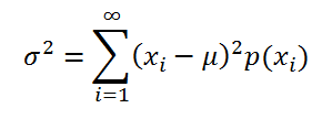
where x i is a value that a random value can take, and μ is the mean value (), p (x) - the probability that the random value will take the value x.

If a random value has, then dispersioncalculated by the formula:

Dimension dispersion corresponds to the square of the unit of measurement of source values. For example, if the values \u200b\u200bin the sample are measuring the weight of the part (in kg), then the dimension of the dispersion will be kg 2. This is difficult to interpret, therefore, for the characteristic of the variation of values, an equal square root from dispersion – standard deviation.

Some properties dispersion:

Var (x + a) \u003d var (x), where x is a random value, and is a constant.

Var (Ah) \u003d a 2 var (x)

Var (x) \u003d e [(xe (x)) 2] \u003d e \u003d e (x 2) -e (2 * x * e (x)) + (E (x)) 2 \u003d e (x 2) - 2 * E (x) * E (x) + (E (x)) 2 \u003d E (x 2) - (E (x)) 2

This dispersion property is used in article about linear regression.

Var (x + y) \u003d var (x) + var (y) + 2 * cov (x; y), where x and y are random variables, cov (x; y) - covariance of these random variables.

If random variables are independent (independent), then them covariator equal to 0, and, therefore, var (x + y) \u003d var (x) + var (y). This dispersion property is used in the output.

We show that for independent variables var (x-y) \u003d var (x + y). Indeed, var (x-y) \u003d var (x-y) \u003d var (x + (- y)) \u003d var (x) + var (-y) \u003d var (x) + var (-y) \u003d var ( X) + (- 1) 2 var (y) \u003d var (x) + var (y) \u003d var (x + y). This dispersion property is used to build.

Standard sample deviation

Standard sample deviation - This is a measure of how wide the values \u200b\u200bin the sample relative to them are scattered.

A-priory, standard deviation equally square root from dispersion:

Standard deviation does not take into account the values \u200b\u200bin sample, but only the degree of dispersion of values \u200b\u200baround them medium. To illustrate this, give an example.

We calculate the standard deviation for 2 samples: (1; 5; 9) and (1001; 1005; 1009). In both cases, S \u003d 4. It is obvious that the ratio of the value of the standard deviation to the values \u200b\u200bof the array at the samples is significantly different. For such cases used The coefficient of variation (Coefficient of Variation, CV) - Standard deviation To medium Arithmetic, pronounced in percent.

In MS Excel 2007 and earlier versions for calculating Standard sample deviation Used function \u003d Standotclone (), eng. Stdev name, i.e. Standard Deviation. From the MS Excel 2010 version, it is recommended to use its analogue \u003d Standotclone.V (), English. name stdev.s, i.e. Sample Standard Deviation.

In addition, starting from the MS Excel 2010 version there is a function of Standotclonal.g (), English. name stdev.p, i.e. Population Standard Deviation, which calculates standard deviation for general aggregate. All the difference is reduced to the denominator: instead of N-1 as a Standotclona.V (), near Standotclone.g () in the denominator, simply n.

Standard deviation You can also calculate directly by the above formulas (see the example file)
\u003d Root (quadroller (sample) / (score (sample) -1))
\u003d Root ((Summkv (sample) -cult (sample) * SRNVOV (sample) ^ 2) / (score (sample) -1))

Other scattering measures

The quadrol () function calculates with ummp squares deviations of values \u200b\u200bfrom their medium. This function will return the same result as the formula \u003d d.g ( Sample)*SCORE( Sample), where Sample- reference to the range containing an array of sampling values \u200b\u200b(). Calculations in the QuadrolC () function are made by the formula:

The syrotchal () function is also a measure of the variation of a plurality of data. Function Slotchal () calculates the average absolute values Deviations of values \u200b\u200bOT medium. This feature will return the same result as the formula \u003d Summipatic (ABS)) / Sampling (sample)where Sample- Link to the range containing an array of sampling values.

Calculations in the Function Function () are manufactured by the formula:

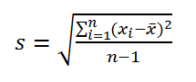
Dispersion is a scattering measure that describes a comparative deviation between data values \u200b\u200band medium size. Is the most used scattering measure in statistics calculated by the summation raised to the square, deviations of each data value from middle size. The formula for calculating the dispersion is presented below:

s 2 - sample dispersion;

x Wed - average sample value;

n. — Sample size (number of data values),

(x i - x cf) - deviation from the average value for each dataset value.

For a better understanding of the formula, we will analyze an example. I do not really love cooking, so the occupation of this is extremely rare. Nevertheless, in order not to die with hunger, from time to time I have to approach the stove to implement the plan on saturation of my organism with proteins, fats and carbohydrates. The data set retood below shows how many times the Renat prepares food every month:

The first step in calculating the dispersion is the definition of the average sampling value, which in our example is 7.8 times a month. The remaining calculations can be facilitated using the following table.

The final phase of the dispersion calculation looks like this:

For those who like to produce all calculations at a time, the equation will look like this:

Using the "Raw Account" method (Example with cooking)

There is more effective method The dispersion calculations known as the "raw account" method. Although at first glance, the equation may seem very cumbersome, in fact it is not terrible. You can make sure this, and then decide which method you like more.

- the sum of each data value after the construction of the square,

- Square amount of all data values.

Do not lose the mind right now. Let me present all this in the form of a table, and then you will see that the calculations here are less than in the previous example.

As you can see, the result turned out the same as when using the previous method. Dignity this method It becomes obvious as the sample size (N) grows.

Excel dispersion calculation

As you already, probably guessed, there is a formula in Excel, which allows you to calculate the dispersion. Moreover, since Excel 2010, you can find 4 varieties of the dispersion formula:

1) Display - returns a sample dispersion. Logical values \u200b\u200band text are ignored.

2) Display - returns dispersion by the general population. Logical values \u200b\u200band text are ignored.

3) Dispa - returns a sample dispersion based on logical and text values.

4) Display - returns dispersion by the general population, taking into account logical and text values.

To begin with, we will understand the difference between the sample and the general population. The purpose of the descriptive statistics is to summarize or display the data so as to quickly receive the overall picture, so to speak, review. Statistical output allows you to make conclusions about any combination based on sampling of data from this totality. The aggregate is all possible outcomes or measurements representing interest to us. The sample is a subset of the aggregate.

For example, we are interested in a totality of a group of students of one of the Russian universities and we need to determine the middle ball of the group. We can calculate the average student performance, and then the resulting digit will be the parameter, since a whole set will be involved in our calculations. However, if we want to calculate the average ball of all students of our country, then this group will be our sample.

The difference in the formula for calculating the dispersion between the sample and the set is the denominator. Where it will be equal to the sample (N-1), and for the general population of only N.

Now we will deal with the functions of calculating the dispersion with the endings BUT,in the description of which it is said that the calculation takes into account text and logical values. In this case, when calculating the dispersion of a specific data array, where there are no numeric values, Excel will interpret text and false logical values \u200b\u200bas equal to 0, and the true logical values \u200b\u200bare equal to 1.

So, if you have an array of data, it is difficult to calculate its dispersion by using one of the above Excel functions.

Theory of probability is a special section of mathematics, which is learn only by students of higher educational institutions. Do you like calculations and formulas? You are not frightened by the prospects of acquaintance with the normal distribution, the entropy of the ensemble, the mathematical expectation and dispersion of the discrete random variable? Then this subject will be very interesting. Let's get acquainted with several essential basic concepts of this section of science.

Recall the basics

Even if you remember the simplest concepts of the theory of probability, do not neglect the first paragraphs of the article. The fact is that without a clear understanding of the basics you will not be able to work with the formulas considered below.

So, there is some random event, a certain experiment. As a result of the actions, we can get several outcomes - some of them are more common, others - less often. The probability of an event is the ratio of the number of actually obtained outcomes of the same type to the total number of possible. Only knowing the classic definition of this concept, you can start learning mathematical expectation and dispersion of continuous random variables.

Average

Still at school in the lessons of mathematics, you started working with an average arithmetic. This concept is widely used in the theory of probability, and therefore it is impossible to bypass the side. The main thing for us on this moment It is that we will face it in the formulas of the mathematical expectation and dispersion of a random variable.

We have a sequence of numbers and want to find the arithmetic average. All that is required from us is to sum up everything available and divided by the number of elements in the sequence. Let we have numbers from 1 to 9. The amount of the elements will be equal to 45, and this value we divide by 9. Answer: - 5.

Dispersion

Speaking scientificDispersion is the average square of deviations of the obtained sign values \u200b\u200bfrom the average arithmetic. It is indicated by one title Latin letter D. What do you need to calculate it? For each element of the sequence, we calculate the difference between the existing number and the average arithmetic and erected into the square. The values \u200b\u200bwill turn out exactly as much as the events considered by us can be. Next, we summarize everything obtained and divided by the number of elements in the sequence. If we have five outcomes, we divide five.

The dispersion has the properties that need to be remembered to apply when solving tasks. For example, with an increase in random variable in X times, the dispersion increases into x in the square times (i.e. x * x). It never happens less than zero and does not depend on the shift of values \u200b\u200bto an equal value in a large or smaller side. In addition, for independent tests, the amount dispersion is equal to the amount of dispersions.

Now we need to consider examples of dispersion of discrete random variance and mathematical expectation.

Suppose we spent 21 experiments and received 7 different outcomes. Each of them we observed, respectively, 1,2,2,3,4,4 and 5 times. What will the dispersion be equal to?

First, consider the arithmetic average: the sum of the elements, of course, is equal to 21. We divide it to 7, yielding 3. Now from each number of the initial sequence will be subtracted 3, each value is erected into a square, and the results will add together together. It turns out 12. Now we have to divide the number on the number of elements, and it would seem, everything. But there is a snag! Let's discuss it.

Dependence on the number of experiments

It turns out that when calculating the dispersion in the denominator may be one of two numbers: either N or N-1. Here n is the number of experiments or the number of elements in the sequence (which is essentially the same). What does it depend on?

If the number of tests is measured by hundreds, then we must put in the N. denominator if units, then N-1. The border scientists decided to hold quite symbolically: today it passes according to the figure 30. If we spent less than 30 experiments, we will divide the amount on N-1, and if more - then on N.

A task

Let's go back to our example solving the problem of dispersion and mathematical expectation. We obtained an intermediate number 12, which it was necessary to divide on n or n-1. Since experiments we conducted 21, which is less than 30, choose the second option. So, the answer: the dispersion is 12/2 \u003d 2.

Expected value

Let us turn to the second concept that we must consider this article. The mathematical expectation is the result of the addition of all possible outcomes, multiplied by the corresponding probabilities. It is important to understand that the value obtained, as well as the result of the dispersion calculation, it turns out only once for a whole task, no matter how outcomes it is not considered.

The formula of the mathematical expectation is quite simple: we take the outcome, multiply on its probability, we add the same for the second, third result, etc. Everything related to this concept is calculated easy. For example, the amount of matchmakers is equal to the sum of the amount. For the work is relevant the same. Such simple operations makes it possible to carry out far from each value in the theory of probability. Let's take the task and consider the importance of the concepts we studied at once. In addition, we were distracted by theory - it's time to practice.

One more example

We spent 50 tests and received 10 types of outcomes - numbers from 0 to 9 - appearing in various percentage. This, respectively: 2%, 10%, 4%, 14%, 2%, 18%, 6%, 16%, 10%, 18%. Recall that in order to obtain probabilities, it is necessary to divide the values \u200b\u200bin percent per 100. Thus, we obtain 0.02; 0.1, etc. Imagine for dispersion of random variance and mathematical expectation example of a solution to the problem.

The arithmetic average is calculated by the formula that I remember from the younger School: 50/10 \u003d 5.

Now we will transfer the probability to the number of outcomes "in pieces" so that it is more convenient to count. We obtain 1, 5, 2, 7, 1, 9, 3, 8, 5, 7, 1, 1, 9, 3, 8, 5, and 9. From each obtained value, the average arithmetic is subtracted, after which each of the results obtained erected into the square. Look how to do this, on the example of the first element: 1 - 5 \u003d (-4). Next: (-4) * (-4) \u003d 16. For the remaining values, do these operations yourself. If you did everything right, then after addition you get 90.

Continue calculating the dispersion and mathematical expectation, dividing 90 on N. Why do we choose n, and not n-1? That's right, because the number of experiments performed exceeds 30. So: 90/10 \u003d 9. The dispersion we received. If you have another number, do not despair. Most likely, you made a banal error when calculating. Check written, and surely everything will fall into place.

Finally, remember the formula of the expectation. We will not give all the calculations, write only the answer you can handle, by completing all the required procedures. Materialization will be equal to 5.48. Recall only how to carry out operations, on the example of the first elements: 0 * 0.02 + 1 * 0,1 ... and so on. As you can see, we simply multiply the value of the outcome of its probability.

Deviation

Another concept, closely associated with dispersion and mathematical expectation - the average quadratic deviation. It is indicated by either Latin SD letters, or a Greek lowercase "sigma". This concept shows how average the values \u200b\u200bfrom the central sign are deflected. To find its meaning, you need to calculate square root From dispersion.

If you build a schedule normal distribution and want to see directly on it quadratic deviationThis can be done in several stages. Take half the image to the left or right of the mode (central value), carry out perpendicular to the horizontal axis so that the area of \u200b\u200bthe figures have been equal. The size of the segment between the middle of the distribution and the resulting projection on the horizontal axis will be a secondary quadratic deviation.

Software

As can be seen from the descriptions of the formulas and the examples presented, the calculations of the dispersion and mathematical expectation are not the simplest procedure from an arithmetic point of view. In order not to spend time, it makes sense to use the program used in the highest educational institutions - It is called "R". It has functions that allow you to calculate the values \u200b\u200bfor many concepts from statistics and probability theory.

For example, you specify the vector values. This is done as follows: vector<-c(1,5,2…). Теперь, когда вам потребуется посчитать какие-либо значения для этого вектора, вы пишете функцию и задаете его в качестве аргумента. Для нахождения дисперсии вам нужно будет использовать функцию var. Пример её использования: var(vector). Далее вы просто нажимаете «ввод» и получаете результат.

Finally

Dispersion and mathematical expectation are without which it is difficult to calculate anything else. In the main year of lectures in universities, they are already considered in the first months of study of the subject. It is because of the misunderstanding of these simplest concepts and inability to calculate them, many students immediately begin to lag behind the program and later get bad marks based on the results of the session, which deprives them of scholarships.

Practice at least one week half an hour per day, solving tasks similar to those presented in this article. Then, on any control on probability theory, you will handle examples without foreign tips and crib.

However, only this characteristic is not enough to study random variance. Imagine two shooters who shoot targets. One shoots a label and gets close to the center, and the other ... just entertained and not even aim. But what's funny, his middle The result will be exactly the same as the first arrow! This situation conventionally illustrates the following random variables:

"Sniper" mathematical expectation is equal, however, a "interesting person": - It is also zero!

Thus, the need arises to quantify how far scattered bullets (random values) relative to the center of the target (mathematical expectation). well and scattering from Latin translates non anyway as dispersion .

Let's see how this numerical characteristic is determined on one example of the 1st part of the lesson:

There we found a disappointing mathematical expectation of this game, and now we have to calculate its dispersion, which denotes through .

We find out how far the "scattered" wins / losses relative to the average value. Obviously, for this you need to calculate difference between values \u200b\u200bof random variable and her mathematical expectation:

–5 – (–0,5) = –4,5
2,5 – (–0,5) = 3
10 – (–0,5) = 10,5

Now it seems to be a summary of the results, but this path is not suitable - for the reason that the oscillations will be interconnected with fluctuations to the right. So, for example, the "amateur" shooter (example above) differences will be And when adding will give zero, so we will not get any estimate of the scattering of its shooting.

To get around this trouble you can consider modules differences, but for technical reasons, approach began when they were erected into a square. The solution is more convenient to place the table:

And here it suggests calculating weighway The value of the squares of deviations. What is it? It's theirs expected valuewhich is the measure of scattering:

– definition Dispersion. From the definition it is immediately clear that dispersion can not be negative - Take note for practice!

We remember how to find a matchmaker. I turn the squares of differences on the corresponding probabilities (Table continuation):
- figuratively speaking, this is "thrust force",
and summarize the results:

Don't you think that against the background of the winnings the result turned out to be Velika? That's right - we were erected in a square, and to return to the dimension of our game, you need to remove the square root. This value is called medium quadratic deviation And indicated by the Greek letter "Sigma":

Sometimes it is called standard deviation .

What is his meaning? If we distinguish from the mathematical expectation to the left and right on the average quadratic deviation:

- This interval will be "concentrated" the most likely values \u200b\u200bof random variance. What we, in fact, are observing:

However, it was so that when analyzing scattering almost always operates with the concept of dispersion. Let's deal with what it means in relation to the games. If, in the case of arrows, we are talking about the "cuminess" of hits with the center of the target, then the dispersion characterizes two things:

First, it is obvious that with increasing rates, the dispersion also increases. For example, if we increase 10 times, the mathematical expectation will increase 10 times, and the dispersion is 100 times (since soon, this is a quadratic value). But, notice that the rules of the game themselves have not changed! Only rates changed, roughly speaking, before we put 10 rubles, now 100.

The second, more interesting moment is that the dispersion characterizes the style of the game. Mentally fix gaming rates at a certain levelAnd let's see what:

Low dispersion game is a careful game. The player is inclined to choose the most reliable schemes, where for 1 time it does not lose / wins too much. For example, the "red / black" system in roulette (See Example 4 Articles Random variables) .

High dispersion game. It is often called it dispersion game. This is an adventurous or aggressive style of the game, where the player chooses "adrenaline" schemes. Recall at least "Martingale"In which the amounts turn out to be the same, for the orders of the preceding "quiet" game of the previous item.

The situation in poker is indicative: there are so-called so-called tighing players who tend to be cautious and "shaking" over your gaming agents (Bankroll). It is not surprising that their bankroll is not subjected to significant fluctuations (low dispersion). On the contrary, if the player has a high dispersion, then this is an aggressor. He often risks, makes large bets and can ride a huge bank and to do in the fluff and dust.

The same thing happens on Forex, and so on - examples of mass.

Moreover, in all cases it does not matter - there is a game on a penny or thousands of dollars. At any level, there are low and highly dispersed players. Well, for the average winnings, as we remember, "answers" expected value.

Probably, you noticed that the dispersion is a long and painstaking process. But Mathematics generous:

Formula for finding dispersion

This formula is displayed directly from the definition of the dispersion, and we immediately let it in turnover. I will copy on top of the table with our game:

And the found matchmaker.

Calculate the dispersion in the second way. We will first find the mathematical expectation - the square of the random variable. By determination of mathematical expectation:

In this case:

Thus, by the formula:

As they say, feel the difference. And in practice, of course, it is better to use the formula (unless otherwise require a condition).

We master the solutions and decoration technique:

Example 6.

Find its mathematical expectation, dispersion and secondary quadratic deviation.

This task is encountered everywhere, and, as a rule, goes without meaningful.
You can imagine several light bulbs with numbers that light up in a madhouse with certain probabilities :)

Decision: The main calculations are convenient to reduce the table. First, in the upper two lines write the source data. Then we calculate the works, then and finally the amounts in the right column:

Actually, almost everything is ready. In the third line, a ready-made mathematical expectation was drawn: .

Dispersion calculated by the formula:

And finally, the average quadratic deviation:
- Personally, I usually round up to 2 signs after the comma.

All calculations can be carried out on the calculator, and even better - in Excele:

here it is already difficult to make a mistake :)

Answer:

Those who wish can easier to simplify their lives and use my calculator (demo)which not only instantly solve this task, but also builds thematic charts (coming soon). The program can be download in the library - If you downloaded at least one educational material, or get another way. Thanks for the support of the project!

A pair of tasks for self solutions:

Example 7.

Calculate the dispersion of the random variable of the previous example by definition.

And similar example:

Example 8.

The discrete random value is given by its distribution law:

Yes, the values \u200b\u200bof random variance are quite large (example from real work), And here, if possible, use Excel. As, by the way, in example 7, it is faster, reliable and more pleasant.

Solutions and answers at the bottom of the page.

In conclusion of the 2nd part of the lesson, we will analyze another model task, you can even say, a small rebus:

Example 9.

Discrete random value can take only two values: and, and. Known is probability, mathematical expectation and dispersion.

Decision: Let's start with an unknown probability. Since the random value can take only two values, then the sum of the probabilities of the respective events:

and since, then.

It remains to find ..., it is easy to say :) But oh well, it suffered. By definition of mathematical expectation:
- We substitute famous values:

- And more from this equation do not squeeze anything, unless you can rewrite it in the usual direction:

or:

About further actions, I think you guess. We will also decide the system:

Decimal fractions are, of course, complete disgrace; Multiply both equations for 10:

and divide on 2:

That's much better. From the 1st equation, we express:
(this is a simpler way)- We substitute in the 2nd equation:

Build in square And we are simplified:

We multiply on:

As a result, received quadratic equation, we find it discriminant:
- well!

and we have two solutions:

1) if T. ;

2) if then.

The condition satisfies the first pair of values. With a high probability, everything is correct, but, nevertheless, write the law of distribution:

And do the check, namely, find a matchmaker: