Remarkable limits and consequences of them. The first wonderful limit

Now with peace of mind, we turn to consideration wonderful limits.
has the form.

Instead of the variable x, various functions can be present, the main thing is that they tend to 0.

The limit needs to be calculated

As you can see, this limit is very similar to the first remarkable one, but this is not entirely true. In general, if you notice sin in the limit, then you should immediately think about whether it is possible to apply the first remarkable limit.

According to our rule # 1, substitute zero for x:

We get uncertainty.

Now let's try to organize the first wonderful limit on our own. To do this, let's use a simple combination:

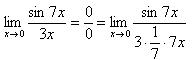
This will arrange the numerator and denominator to highlight 7x. The familiar, wonderful limit has already emerged. It is advisable to highlight it when deciding:

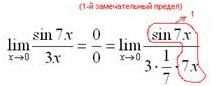
Let us substitute the solution of the first wonderful example and we get:

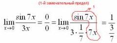
Simplifying the fraction:

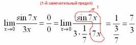
Answer: 7/3.

As you can see, everything is very simple.

Has the form where e = 2.718281828 ... is an irrational number.

Instead of the variable x, various functions can be present, the main thing is that they strive for.

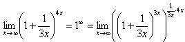
The limit needs to be calculated

Here we see the presence of a degree under the sign of the limit, which means that the application of the second remarkable limit is possible.

As always, we will use rule number 1 - substitute for x:

It can be seen that for x the base of the degree, and the exponent is 4x>, i.e. we get an uncertainty of the form:

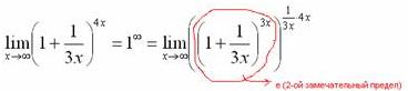
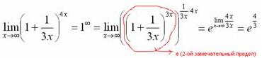
Let's use the second wonderful limit to reveal our uncertainty, but first we need to organize it. As you can see, it is necessary to achieve presence in the indicator, for which we raise the base to the power of 3x, and at the same time to the power of 1 / 3x, so that the expression does not change:

Do not forget to highlight our wonderful limit:

These are really wonderful limits!
If you still have any questions about the first and second wonderful limits, then feel free to ask them in the comments.
We will answer everyone if possible.

You can also work with a teacher on this topic.
We are pleased to offer you the services of selecting a qualified tutor in your city. Our partners will promptly select a good teacher for you on favorable terms.

Not enough information? - You can !

You can write mathematical calculations in notebooks. It is much more pleasant for individuals to write in notebooks with a logo (http://www.blocnot.ru).

Find wonderful limits it is difficult not only for many first and second year students who study the theory of limits, but also for some teachers.

Formula for the first remarkable limit

Consequences of the first remarkable limit can be written by the formulas
1. 2. 3. 4. But by themselves, the general formulas of remarkable limits do not help anyone on an exam or test. The bottom line is that real tasks are built so that you still need to come to the formulas written above. And most of the students who miss the pairs, study this course by correspondence or have teachers who themselves do not always understand what they are explaining, cannot calculate the most elementary examples to remarkable limits. From the formulas of the first remarkable limit, we see that they can be used to investigate uncertainties of the type zero divided by zero for expressions with trigonometric functions. Let's first look at a number of examples for the first remarkable limit, and then explore the second remarkable limit.

Example 1. Find the limit of the function sin (7 * x) / (5 * x)
Solution: As you can see, the function under the limit is close to the first remarkable limit, but the limit of the function itself is definitely not equal to one. In this kind of tasks for the limits, you should select the variable in the denominator with the same coefficient that is contained in the variable under the sine. In this case, divide and multiply by 7

To some, such detailing will seem superfluous, but for most students who find it difficult to give limits, it will help to better understand the rules and learn theoretical material.
Also, if there is a reverse kind of function, this is also the first remarkable limit. And all because the wonderful limit is one

The same rule applies to consequences of 1 remarkable limit. Therefore, if you are asked "What is the first wonderful limit?" You must answer without hesitation that it is one.

Example 2. Find the limit of the function sin (6x) / tan (11x)
Solution: To understand the final result, let's write the function in the form

To apply the rules of the remarkable limit, we multiply and divide by factors

Further, we write the limit of the product of functions in terms of the product of the limits

Without complicated formulas, we have found the limit of the hour trigonometric functions... For assimilation simple formulas try to come up with and find the limit on 2 and 4 the formula of Corollary 1 of the remarkable limit. We'll look at more complex tasks.

Example 3. Calculate the limit (1-cos (x)) / x ^ 2
Solution: When checking by substitution, we get an uncertainty of 0/0. Many people do not know how to reduce such an example to one remarkable limit. The trigonometric formula should be used here

In this case, the limit will be transformed to an understandable form

We have succeeded in reducing the function to the square of a remarkable limit.

Example 4. Find the limit
Solution: Substitution gives the familiar 0/0 feature. However, the variable tends to Pi, not zero. Therefore, to apply the first remarkable limit, we change the variable x so that the new variable goes to zero. To do this, denote the denominator as a new variable Pi-x = y

Thus, using the trigonometric formula, which is given in the previous task, the example is reduced to 1 remarkable limit.

Example 5. Calculate the limit
Solution: At first, it is not clear how to simplify the limits. But since there is an example, then there must be an answer. The fact that the variable is directed to one gives, when substituted, a singularity of the form zero multiplied by infinity, so the tangent must be replaced by the formula

After that, we get the desired uncertainty 0/0. Next, we perform the change of variables in the limit, and use the periodicity of the cotangent

The last substitutions allow us to use Corollary 1 of the remarkable limit.

The second remarkable limit is exponential

This is a classic to which in real problems it is not always easy to reach the limits.
In calculations you will need limits are consequences of the second remarkable limit:
1. 2. 3. 4.
Thanks to the second remarkable limit and its consequences, it is possible to study uncertainties such as zero divided by zero, one to the power of infinity, and infinity divided by infinity, and even to the same degree.

Let's start to get familiar with simple examples.

Example 6. Find the limit of a function
Solution: You cannot directly apply the 2 wonderful limit. First, you should turn the exponent so that it has the opposite form to the term in parentheses

This is the technique of reducing to the 2 remarkable limit and, in fact, the derivation 2 of the formula for the corollary of the limit.

Example 7. Find the limit of a function
Solution: We have tasks for 3 the formula of Corollary 2 of a remarkable limit. Substitution of zero gives a feature of the form 0/0. To raise the limit under the rule, turn the denominator so that the variable has the same coefficient as in the logarithm

It is also easy to understand and accomplish on the exam. Students' difficulty in calculating limits begins with the following tasks.

Example 8. Calculate the limit of a function[(x + 7) / (x-3)] ^ (x-2)
Solution: We have a singularity of type 1 to the degree of infinity. If you do not believe, you can substitute infinity instead of "X" everywhere and make sure of it. To build under the rule, divide the numerator by the denominator in parentheses, for this we first perform the manipulations

Substitute the expression into the limit and turn to 2 the remarkable limit

The limit is exponential to the 10th power. Constants, which are addends for a variable both in brackets and a degree, do not bring any "weather" - this should be remembered. And if the teachers ask you - "Why don't you turn the indicator?" (For this example in x-3), then say that "When a variable tends to infinity, then at least add 100 to it, or subtract 1000, and the limit will remain the same!".
There is a second way to calculate these types of limits. We will talk about it in the next task.

Example 9. Find the limit
Solution: Now let's move out the variable in the numerator and denominator and convert one feature to another. To obtain the final value, we use the formula of Corollary 2 of the remarkable limit

Example 10. Find the limit of a function
Solution: Not everyone can find the set limit. To raise the limit under 2, imagine that sin (3x) is a variable, but you need to turn the exponent

Further, the indicator will be written as a degree to a degree


Intermediate reasoning is described in parentheses. As a result of using the first and second remarkable limit, we got an exponent in a cube.

Example 11. Calculate the limit of a function sin (2 * x) / ln (3 * x + 1)
Solution: We have an uncertainty of the form 0/0. In addition, we see that the function should be converted to use both remarkable limits. Let's perform the previous mathematical transformations

Further, without difficulty, the limit will take on the value

This is how you will feel at ease on examinations, tests, modules if you learn to quickly describe functions and bring them under the first or second wonderful limit. If it is difficult for you to memorize the given methods of finding the limits, then you can always order test to our limits.
To do this, fill out the form, specify the data and attach a file with examples. We have helped many students - we can help you too!

Proof:

First, we prove the theorem for the case of the sequence

According to the binomial Newton formula:

Assuming we get

From this equality (1) it follows that as n increases, the number of positive terms on the right-hand side increases. In addition, as n increases, the number decreases, so the quantities increase. Therefore, the sequence increasing, while (2) * Let us show that it is bounded. Replace each parenthesis on the right side of the equality with one, right part increases, we obtain the inequality

Let's strengthen the resulting inequality, replace 3,4,5, ..., standing in the denominators of fractions, with the number 2: The sum in parentheses is found by the formula for the sum of the terms of a geometric progression: Therefore (3)*

So, the sequence is bounded from above, while inequalities (2) and (3) hold: Therefore, based on the Weierstrass theorem (a criterion for the convergence of a sequence), the sequence monotonically increasing and limited, which means it has a limit, denoted by the letter e. Those.

Knowing that the second remarkable limit is true for natural values ​​of x, we prove the second remarkable limit for real x, that is, we will prove that ... Consider two cases:

1. Let Each value of x be enclosed between two positive integers:, where is whole part x. => =>

If, then Therefore, according to the limit We have

On the basis (about the limit of the intermediate function) of the existence of the limits

2. Let. We make the substitution - x = t, then

From these two cases it follows that for real x.

Consequences:

9 .) Comparison of infinitesimal. The theorem on the replacement of infinitesimal by equivalent in the limit and the theorem on the principal part of the infinitesimal.

Let the functions a ( x) and b ( x) - b.m. at x ® x 0 .

DEFINITIONS.

1) a ( x) called infinitesimal of higher order than b (x) if

Write: a ( x) = o (b ( x)) .

2) a ( x) and b ( x)are called infinitesimal of the same order, if

where CÎℝ and C¹ 0 .

Write: a ( x) = O(b ( x)) .

3) a ( x) and b ( x) are called equivalent , if

Write: a ( x) ~ b ( x).

4) a ( x) is called infinitesimal of order k with respect to
infinitely small b ( x), if infinitesimal a ( x)and(b ( x)) k are of the same order, i.e. if

where CÎℝ and C¹ 0 .

THEOREM 6 (on the replacement of infinitesimal by equivalent).

Let be a ( x), b ( x), a 1 ( x), b 1 ( x)- b.m. at x ® x 0 ... If a ( x) ~ a 1 ( x), b ( x) ~ b 1 ( x),

then

Proof: Let a ( x) ~ a 1 ( x), b ( x) ~ b 1 ( x), then

THEOREM 7 (about the main part of the infinitesimal).

Let be a ( x)and b ( x)- b.m. at x ® x 0 , and b ( x)- b.m. higher order than a ( x).

=, a since b ( x) - of a higher order than a ( x), then, i.e. from it is clear that a ( x) + b ( x) ~ a ( x)

10) Continuity of a function at a point (in the language of epsilon-delta limits, geometric) One-sided continuity. Continuity on an interval, on a segment. Properties of continuous functions.

1. Basic definitions

Let be f(x) is defined in some neighborhood of the point x 0 .

DEFINITION 1. Function f(x) called continuous at point x 0 if the equality is true

Remarks.

1) By virtue of Theorem 5 §3, equality (1) can be written in the form

Condition (2) - definition of the continuity of a function at a point in the language of one-sided limits.

2) Equality (1) can also be written as:

They say: “if the function is continuous at the point x 0, then the sign of the limit and the function can be reversed. "

DEFINITION 2 (in language e-d).

Function f(x) called continuous at point x 0 if"e> 0 $ d> 0 such, what

if xÎU ( x 0, d) (i.e. | x – x 0 | < d),

then f(x) ÎU ( f(x 0), e) (i.e. | f(x) – f(x 0) | < e).

Let be x, x 0 Î D(f) (x 0 - fixed, x - arbitrary)

We denote: D x= x - x 0 – argument increment

D f(x 0) = f(x) – f(x 0) – function increment at point x 0

DEFINITION 3 (geometric).

Function f(x) on called continuous at point x 0 if at this point the infinitesimal increment of the argument corresponds to the infinitesimal increment of the function, i.e.

Let the function f(x) is defined on the interval [ x 0 ; x 0 + d) (on the interval ( x 0 - d; x 0 ]).

DEFINITION. Function f(x) called continuous at point x 0 on right (left ), if the equality is true

It's obvious that f(x) is continuous at the point x 0 Û f(x) is continuous at the point x 0 right and left.

DEFINITION. Function f(x) called continuous for an interval e ( a; b) if it is continuous at every point of this interval.

Function f(x) is called continuous on the segment [a; b] if it is continuous on the interval (a; b) and has one-sided continuity at the boundary points(i.e., is continuous at the point a on the right, at the point b- left).

11) Break points, their classification

DEFINITION. If the function f(x) defined in some neighborhood of the point x 0 , but is not continuous at this point, then f(x) is called discontinuous at the point x 0 , but the point itself x 0 called a break point function f(x) .

Remarks.

1) f(x) can be defined in an incomplete neighborhood of the point x 0 .

Then the corresponding one-sided continuity of the function is considered.

2) From the definition of Þ point x 0 is the discontinuity point of the function f(x) in two cases:

a) U ( x 0, d) Î D(f) , but for f(x) the equality

b) U * ( x 0, d) Î D(f) .

For elementary functions only case b) is possible.

Let be x 0 - function break point f(x) .

DEFINITION. Point x 0 called break point I kind if the function f(x)has finite limits on the left and right at this point.

If, in addition, these limits are equal, then the point x 0 called point of removable discontinuity , otherwise - jump point .

DEFINITION. Point x 0 called break point II kind if at least one of the one-sided limits of the function f(x)at this point is¥ or does not exist.

12) Properties of functions continuous on an interval (theorems of Weierstrass (without proof) and Cauchy

Weierstrass theorem

Let the function f (x) be continuous on an interval, then

1) f (x) is bounded on

2) f (x) takes its smallest and largest value on the interval

Definition: The value of the function m = f is called the smallest if m≤f (x) for any x € D (f).

The value of the function m = f is called the largest if m≥f (x) for any x ∈ D (f).

The function can take the smallest \ largest value at several points of the segment.

f (x 3) = f (x 4) = max

Cauchy's theorem.

Let the function f (x) be continuous on an interval and x is a number between f (a) and f (b), then there exists at least one point x 0 € such that f (x 0) = g

This article: "The second remarkable limit" is devoted to disclosure within the uncertainties of the form:

$ \ bigg [\ frac (\ infty) (\ infty) \ bigg] ^ \ infty $ and $ ^ \ infty $.

Also, such uncertainties can be disclosed using the logarithm of the exponential power function, but this is already a different solution method, which will be covered in another article.

Formula and Consequences

Formula the second remarkable limit is written as follows: $$ \ lim_ (x \ to \ infty) \ bigg (1+ \ frac (1) (x) \ bigg) ^ x = e, \ text (where) e \ approx 2.718 $$

The formula implies consequences, which are very convenient to use for solving examples with limits: $$ \ lim_ (x \ to \ infty) \ bigg (1 + \ frac (k) (x) \ bigg) ^ x = e ^ k, \ text (where) k \ in \ mathbb (R) $$ $$ \ lim_ (x \ to \ infty) \ bigg (1 + \ frac (1) (f (x)) \ bigg) ^ (f (x)) = e $ $ $$ \ lim_ (x \ to 0) \ bigg (1 + x \ bigg) ^ \ frac (1) (x) = e $$

It is worth noting that the second remarkable limit can be applied not always to the exponential function, but only in cases where the base tends to unity. To do this, first, the base limit is calculated in the mind, and then conclusions are drawn. All of this will be covered in the sample solutions.

Examples of solutions

Let's consider examples of solutions using the direct formula and its consequences. We will also analyze the cases in which the formula is not needed. It is enough to write down only the ready-made answer.

Example 1

Find the limit $ \ lim_ (x \ to \ infty) \ bigg (\ frac (x + 4) (x + 3) \ bigg) ^ (x + 3) $

Solution

Let's substitute infinity in the limit and look at the uncertainty: $$ \ lim_ (x \ to \ infty) \ bigg (\ frac (x + 4) (x + 3) \ bigg) ^ (x + 3) = \ bigg (\ frac (\ infty) (\ infty) \ bigg) ^ \ infty $$ Find the limit of the base: $$ \ lim_ (x \ to \ infty) \ frac (x + 4) (x + 3) = \ lim_ (x \ to \ infty) \ frac (x (1+ \ frac (4) ( x))) (x (1+ \ frac (3) (x))) = 1 $$ We got a base equal to one, which means that the second remarkable limit can already be applied. To do this, we fit the base of the function to the formula by subtracting and adding one: $$ \ lim_ (x \ to \ infty) \ bigg (1 + \ frac (x + 4) (x + 3) - 1 \ bigg) ^ (x + 3) = \ lim_ (x \ to \ infty) \ bigg (1 + \ frac (1) (x + 3) \ bigg) ^ (x + 3) = $$ We look at the second consequence and write down the answer: $$ \ lim_ (x \ to \ infty) \ bigg (1 + \ frac (1) (x + 3) \ bigg) ^ (x + 3) = e $$ If you can't solve your problem, then send it to us. We will provide detailed solution... You will be able to familiarize yourself with the course of the calculation and get information. This will help you get credit from the teacher in a timely manner!

Answer

$$ \ lim_ (x \ to \ infty) \ bigg (1 + \ frac (1) (x + 3) \ bigg) ^ (x + 3) = e $$

Example 4

Solve limit $ \ lim_ (x \ to \ infty) \ bigg (\ frac (3x ^ 2 + 4) (3x ^ 2-2) \ bigg) ^ (3x) $

Solution

We find the limit of the base and see that $ \ lim_ (x \ to \ infty) \ frac (3x ^ 2 + 4) (3x ^ 2-2) = 1 $, so the second wonderful limit can be applied. Standardly, according to the plan, we add and subtract one from the base of the degree: $$ \ lim_ (x \ to \ infty) \ bigg (1+ \ frac (3x ^ 2 + 4) (3x ^ 2-2) -1 \ bigg) ^ (3x) = \ lim_ (x \ to \ infty ) \ bigg (1+ \ frac (6) (3x ^ 2-2) \ bigg) ^ (3x) = $$ We adjust the fraction to the formula of the 2nd remark. limit: $$ = \ lim_ (x \ to \ infty) \ bigg (1+ \ frac (1) (\ frac (3x ^ 2-2) (6)) \ bigg) ^ (3x) = $$ Now we adjust the degree. The power must be a fraction equal to the denominator of the base $ \ frac (3x ^ 2-2) (6) $. To do this, multiply and divide the degree by it, and continue to solve: $$ = \ lim_ (x \ to \ infty) \ bigg (1+ \ frac (1) (\ frac (3x ^ 2-2) (6)) \ bigg) ^ (\ frac (3x ^ 2-2) (6) \ cdot \ frac (6) (3x ^ 2-2) \ cdot 3x) = \ lim_ (x \ to \ infty) e ^ (\ frac (18x) (3x ^ 2-2)) = $$ The limit located in degree at $ e $ is: $ \ lim_ (x \ to \ infty) \ frac (18x) (3x ^ 2-2) = 0 $. Therefore, continuing the solution, we have:

Answer

$$ \ lim_ (x \ to \ infty) \ bigg (\ frac (3x ^ 2 + 4) (3x ^ 2-2) \ bigg) ^ (3x) = 1 $$

Let us examine the cases when the problem is similar to the second remarkable limit, but it can be solved without it.

In the article: "The second remarkable limit: examples of solutions" was analyzed the formula, its consequences and given the frequent types of problems on this topic.

The formula for the second remarkable limit is lim x → ∞ 1 + 1 x x = e. Another notation looks like this: lim x → 0 (1 + x) 1 x = e.

When we talk about the second remarkable limit, we have to deal with an uncertainty of the form 1 ∞, i.e. a unit to an infinite degree.

Yandex.RTB R-A-339285-1

Consider problems in which the ability to calculate the second remarkable limit will come in handy.

Example 1

Find the limit lim x → ∞ 1 - 2 x 2 + 1 x 2 + 1 4.

Solution

Substitute the desired formula and perform the calculations.

lim x → ∞ 1 - 2 x 2 + 1 x 2 + 1 4 = 1 - 2 ∞ 2 + 1 ∞ 2 + 1 4 = 1 - 0 ∞ = 1 ∞

In our answer, we got one to the power of infinity. To determine the solution method, we use the uncertainty table. Let's choose the second remarkable limit and make a change of variables.

t = - x 2 + 1 2 ⇔ x 2 + 1 4 = - t 2

If x → ∞, then t → - ∞.

Let's see what we got after the replacement:

lim x → ∞ 1 - 2 x 2 + 1 x 2 + 1 4 = 1 ∞ = lim x → ∞ 1 + 1 t - 1 2 t = lim t → ∞ 1 + 1 t t - 1 2 = e - 1 2

Answer: lim x → ∞ 1 - 2 x 2 + 1 x 2 + 1 4 = e - 1 2.

Example 2

Compute the limit lim x → ∞ x - 1 x + 1 x.

Solution

Substitute infinity and get the following.

lim x → ∞ x - 1 x + 1 x = lim x → ∞ 1 - 1 x 1 + 1 x x = 1 - 0 1 + 0 ∞ = 1 ∞

In the answer, we again got the same thing as in the previous problem, therefore, we can again use the second remarkable limit. Next, we need to select the whole part at the base of the power function:

x - 1 x + 1 = x + 1 - 2 x + 1 = x + 1 x + 1 - 2 x + 1 = 1 - 2 x + 1

After that, the limit takes the following form:

lim x → ∞ x - 1 x + 1 x = 1 ∞ = lim x → ∞ 1 - 2 x + 1 x

We replace the variables. Suppose that t = - x + 1 2 ⇒ 2 t = - x - 1 ⇒ x = - 2 t - 1; if x → ∞, then t → ∞.

After that, we write down what we got in the original limit:

lim x → ∞ x - 1 x + 1 x = 1 ∞ = lim x → ∞ 1 - 2 x + 1 x = lim x → ∞ 1 + 1 t - 2 t - 1 = = lim x → ∞ 1 + 1 t - 2 t 1 + 1 t - 1 = lim x → ∞ 1 + 1 t - 2 t lim x → ∞ 1 + 1 t - 1 = = lim x → ∞ 1 + 1 tt - 2 1 + 1 ∞ = e - 2 (1 + 0) - 1 = e - 2

To perform this transformation, we used the basic properties of limits and degrees.

Answer: lim x → ∞ x - 1 x + 1 x = e - 2.

Example 3

Find the limit lim x → ∞ x 3 + 1 x 3 + 2 x 2 - 1 3 x 4 2 x 3 - 5.

Solution

lim x → ∞ x 3 + 1 x 3 + 2 x 2 - 1 3 x 4 2 x 3 - 5 = lim x → ∞ 1 + 1 x 3 1 + 2 x - 1 x 3 3 2 x - 5 x 4 = = 1 + 0 1 + 0 - 0 3 0 - 0 = 1 ∞

After that, we need to transform the function to apply the second remarkable limit. We got the following:

lim x → ∞ x 3 + 1 x 3 + 2 x 2 - 1 3 x 4 2 x 3 - 5 = 1 ∞ = lim x → ∞ x 3 - 2 x 2 - 1 - 2 x 2 + 2 x 3 + 2 x 2 - 1 3 x 4 2 x 3 - 5 = = lim x → ∞ 1 + - 2 x 2 + 2 x 3 + 2 x 2 - 1 3 x 4 2 x 3 - 5

lim x → ∞ 1 + - 2 x 2 + 2 x 3 + 2 x 2 - 1 3 x 4 2 x 3 - 5 = lim x → ∞ 1 + - 2 x 2 + 2 x 3 + 2 x 2 - 1 x 3 + 2 x 2 - 1 - 2 x 2 + 2 - 2 x 2 + 2 x 3 + 2 x 2 - 1 3 x 4 2 x 3 - 5 = = lim x → ∞ 1 + - 2 x 2 + 2 x 3 + 2 x 2 - 1 x 3 + 2 x 2 - 1 - 2 x 2 + 2 - 2 x 2 + 2 x 3 + 2 x 2 - 1 3 x 4 2 x 3 - 5

Since now we have the same exponents in the numerator and denominator of the fraction (equal to six), the limit of the fraction at infinity will be equal to the ratio of these coefficients at the highest powers.

lim x → ∞ 1 + - 2 x 2 + 2 x 3 + 2 x 2 - 1 x 3 + 2 x 2 - 1 - 2 x 2 + 2 - 2 x 2 + 2 x 3 + 2 x 2 - 1 3 x 4 2 x 3 - 5 = = lim x → ∞ 1 + - 2 x 2 + 2 x 3 + 2 x 2 - 1 x 3 + 2 x 2 - 1 - 2 x 2 + 2 - 6 2 = lim x → ∞ 1 + - 2 x 2 + 2 x 3 + 2 x 2 - 1 x 3 + 2 x 2 - 1 - 2 x 2 + 2 - 3

Replacing t = x 2 + 2 x 2 - 1 - 2 x 2 + 2 gives us a second remarkable limit. Means what:

lim x → ∞ 1 + - 2 x 2 + 2 x 3 + 2 x 2 - 1 x 3 + 2 x 2 - 1 - 2 x 2 + 2 - 3 = lim x → ∞ 1 + 1 tt - 3 = e - 3

Answer: lim x → ∞ x 3 + 1 x 3 + 2 x 2 - 1 3 x 4 2 x 3 - 5 = e - 3.

conclusions

Uncertainty 1 ∞, i.e. one to an infinite degree is a power uncertainty, therefore, it can be expanded using the rules for finding the limits of exponential functions.

If you notice an error in the text, please select it and press Ctrl + Enter