Solving equations of higher degrees in various ways. Equations of higher degrees

"Methods for solving equations of higher degrees"

( Kiselev readings)

Mathematics teacher Afanasyeva L.A.

MKOU Verkhnekarachanskaya secondary school

Gribanovsky district, Voronezh region

2015 year

Mathematical education received in a comprehensive school is an essential component of general education and the general culture of modern man.

The famous German mathematician Courant wrote: "For over two millennia, the possession of some, not too superficial, knowledge in the field of mathematics has been a necessary component in the intellectual inventory of every educated person." And among this knowledge, the last place belongs to the ability to solve equations.

Already in ancient times, people realized how important it is to learn how to solve algebraic equations. About 4,000 years ago, Babylonian scholars mastered the solution of the quadratic equation and solved systems of two equations, of which one is of the second degree. With the help of equations, various problems of land surveying, architecture and military affairs were solved, many and various questions of practice and natural science were reduced to them, since the exact language of mathematics allows you to simply express facts and relationships, which, when set out in ordinary language, may seem confusing and complex. The equation is one of the most important concepts of mathematics. The development of methods for solving equations, starting with the emergence of mathematics as a science, has long been the main subject of the study of algebra. And today, in mathematics lessons, starting from the first stage of training, much attention is paid to solving equations of various kinds.

There is no universal formula for finding the roots of an algebraic equation of degree n. Many, of course, had the tempting idea to find for any degree n formulas that express the roots of the equation in terms of its coefficients, that is, they solve the equation in radicals. However, the “gloomy Middle Ages” turned out to be as gloomy as possible with regard to the problem under discussion - for the whole seven centuries no one has found the required formulas! Only in the 16th century did Italian mathematicians move forward - to find formulas for n =3 and n =4 . At the same time, the issue of the general solution of equations of the 3rd degree was dealt with by Scipio Dal Ferro, his student Fiori and Tartaglia. In 1545, the book of the Italian mathematician D Cardano, Great Art, or On the Rules of Algebra, was published, where along with other questions of algebra, general methods for solving cubic equations are considered, as well as a method for solving equations of the 4th degree, discovered by his student L. Ferrari. A complete statement of the questions connected with the solution of equations of the 3rd and 4th degrees was given by F. Viet. And in the 20s of the 19th century, the Norwegian mathematician N. Abel proved that the roots of equations of the 5th and higher degrees cannot be expressed through radicals.

The process of finding solutions to an equation usually consists in replacing the equation with an equivalent one. Replacing the equation with equivalent is based on the use of four axioms:

1. If equal values \u200b\u200bare increased by the same number, then the results will be equal.

2. If one and the same number are subtracted from equal values, the results will be equal.

3. If equal values \u200b\u200bare multiplied by the same number, then the results will be equal.

4. If equal values \u200b\u200bare divided by the same number, then the results will be equal.

Since the left side of the equation P (x) \u003d 0 is an nth polynomial, it is useful to recall the following statements:

Statements about the roots of the polynomial and its divisors:

1. A polynomial of degree n has a number of roots that does not exceed number n, and roots of multiplicity m occur exactly m times.

2. An odd degree polynomial has at least one real root.

3. If α is the root of P (x), then P n (x) \u003d (x - α) · Q n - 1 (x), where Q n - 1 (x) is a polynomial of degree (n - 1).

4. Every integer root of a polynomial with integer coefficients is a divisor of the free term.

5. The reduced polynomial with integer coefficients cannot have fractional rational roots.

6. For a polynomial of the third degree

P 3 (x) \u003d ax 3 + bx 2 + cx + d one of the two is possible: either it decomposes into the product of three binomials

P 3 (x) \u003d a (x - α) (x - β) (x - γ), or decomposes into the product of the binomial and the square trinomial P 3 (x) \u003d a (x - α) (x 2 + βx + γ )

7. Any fourth-degree polynomial decomposes into a product of two square trinomials.

8. The polynomial f (x) is divisible by the polynomial g (x) without remainder if there exists a polynomial q (x) such that f (x) \u003d g (x) · q (x). For division of polynomials, the “division by corner” rule applies.

9. For the polynomial P (x) to be divisible by the binomial (x - c), it is necessary and sufficient that P (x) be a root (Corollary to Bezout's theorem).

10. Vieta's theorem: If x 1, x 2, ..., x n are the real roots of the polynomial

P (x) \u003d a 0 x n + a 1 x n - 1 + ... + a n, then the following equalities hold:

x 1 + x 2 + ... + x n \u003d -a 1 / a 0,

x 1 · x 2 + x 1 · x 3 + ... + x n - 1 · x n \u003d a 2 / a 0,

x 1 · x 2 · x 3 + ... + x n - 2 · x n - 1 · x n \u003d -a 3 / a 0,

x 1 · x 2 · x 3 · x n \u003d (-1) n a n / a 0.

Solution Examples

Example 1 . Find the remainder of the division of P (x) \u003d x 3 + 2/3 x 2 - 1/9 by (x - 1/3).

Decision. By the corollary of Bezout’s theorem: “The remainder of dividing a polynomial by a binomial (x - c) is equal to the value of the polynomial in c”. We find P (1/3) \u003d 0. Therefore, the remainder is 0 and the number 1/3 is the root of the polynomial.

Answer: R \u003d 0.

Example 2 . Divide the "corner" 2x 3 + 3x 2 - 2x + 3 by (x + 2). Find the remainder and the partial quotient.

Decision:

2x 3 + 3x 2 - 2x + 3 | x + 2

2x 3 + 4x 2 2x 2 - x

X 2 - 2x

Answer: R \u003d 3; quotient: 2x 2 - x.

Basic methods for solving equations of higher degrees

1. Introduction of a new variable

The method of introducing a new variable is that to solve the equation f (x) \u003d 0, introduce a new variable (substitution) t \u003d xn or t \u003d g (x) and express f (x) in terms of t, obtaining a new equation r (t) . Solving then the equation r (t), find the roots: (t 1, t 2, ..., t n). After that, a set of n equations q (x) \u003d t 1, q (x) \u003d t 2, ..., q (x) \u003d t n is obtained, from which the roots of the original equation are found.

Example; (x 2 + x + 1) 2 - 3x 2 - 3x - 1 \u003d 0.

Solution: (x 2 + x + 1) 2 - 3x 2 - 3x - 1 \u003d 0.

(x 2 + x + 1) 2 - 3 (x 2 + x + 1) + 3 - 1 \u003d 0.

Replacement (x 2 + x + 1) \u003d t.

t 2 - 3t + 2 \u003d 0.

t 1 \u003d 2, t 2 \u003d 1. Reverse replacement:

x 2 + x + 1 \u003d 2 or x 2 + x + 1 \u003d 1;

x 2 + x - 1 \u003d 0 or x 2 + x \u003d 0;

From the first equation: x 1, 2 \u003d (-1 ± √5) / 2, from the second: 0 and -1.

The method of introducing a new variable finds application in solving returnable equations, that is, equations of the form a 0 x n + a 1 x n - 1 + .. + a n - 1 x + a n \u003d 0, in which the coefficients of the terms of the equation equally spaced from the beginning and end are equal.

2. Factorization by grouping and shorthand multiplication formulas

The basis of this method is to group the terms so that each group contains a common factor. To do this, sometimes you have to apply some artificial tricks.

Example: x 4 - 3x 2 + 4x - 3 \u003d 0.

Decision. Imagine - 3x 2 \u003d -2x 2 - x 2 and group:

(x 4 - 2x 2) - (x 2 - 4x + 3) \u003d 0.

(x 4 - 2x 2 +1 - 1) - (x 2 - 4x + 3 + 1 - 1) \u003d 0.

(x 2 - 1) 2 - 1 - (x - 2) 2 + 1 \u003d 0.

(x 2 - 1) 2 - (x - 2) 2 \u003d 0.

(x 2 - 1 - x + 2) (x 2 - 1 + x - 2) \u003d 0.

(x 2 - x + 1) (x 2 + x - 3) \u003d 0.

x 2 - x + 1 \u003d 0 or x 2 + x - 3 \u003d 0.

There are no roots in the first equation, from the second: x 1, 2 \u003d (-1 ± √13) / 2.

3. Factorization by the method of indefinite coefficients

The essence of the method is that the original polynomial is factorized with unknown coefficients. Using the property that polynomials are equal if their coefficients are equal at the same degrees, unknown expansion coefficients are found.

Example: x 3 + 4x 2 + 5x + 2 \u003d 0.

Decision. A polynomial of degree 3 can be decomposed into a product of linear and square factors.

x 3 + 4x 2 + 5x + 2 \u003d (x - a) (x 2 + bx + c),

x 3 + 4x 2 + 5x + 2 \u003d x 3 + bx 2 + cx - ax 2 - abx - ac,

x 3 + 4x 2 + 5x + 2 \u003d x 3 + (b - a) x 2 + (c - ab) x - ac.

Having solved the system:

we get

x 3 + 4x 2 + 5x + 2 \u003d (x + 1) (x 2 + 3x + 2).

The roots of the equation (x + 1) (x 2 + 3x + 2) \u003d 0 are easily found.

Answer: -1; -2.

4. Method of root selection by senior and free coefficient

The method relies on the application of theorems:

1) Every integer root of a polynomial with integer coefficients is a divisor of a free term.

2) In order for the irreducible fraction p / q (p is an integer, q is a positive integer) to be the root of the equation with integer coefficients, it is necessary that the number p be the integer divisor of the free term a 0, and q is the natural divisor of the highest coefficient.

Example: 6x 3 + 7x 2 - 9x + 2 \u003d 0.

Decision:

2: p \u003d ± 1, ± 2

6: q \u003d 1, 2, 3, 6.

Therefore, p / q \u003d ± 1, ± 2, ± 1/2, ± 1/3, ± 2/3, ± 1/6.

Having found one root, for example - 2, we will find other roots using angle division, the method of indefinite coefficients or Horner's scheme.

Answer: -2; 1/2; 1/3.

5. The graphical method.

This method consists in plotting and using the properties of functions.

Example: x 5 + x - 2 \u003d 0

We represent the equation in the form x 5 \u003d - x + 2. The function y \u003d x 5 is increasing, and the function y \u003d - x + 2 is decreasing. Therefore, the equation x 5 + x - 2 \u003d 0 has a single root of -1.

6. Multiplication of the equation by a function.

Sometimes the solution of an algebraic equation is greatly facilitated if you multiply both its parts by some function - a polynomial from an unknown. It should be remembered that the appearance of extra roots is possible - the roots of the polynomial by which the equation is multiplied. Therefore, one must either multiply by a polynomial that does not have roots and obtain an equivalent equation, or multiply by a polynomial that has roots, and then each of these roots must be substituted into the original equation and establish whether this number is its root.

Example. Solve the equation:

X 8 - X 6 + X 4 - X 2 + 1 \u003d 0. (1)

Decision: Multiplying both sides of the equation by the polynomial X 2 + 1, which has no roots, we obtain the equation:

(X 2 +1) (X 8 - X 6 + X 4 - X 2 + 1) \u003d 0 (2)
equivalent to equation (1). Equation (2) can be written as:

X 10 + 1 \u003d 0 (3)
It is clear that equation (3) has no real roots, therefore equation (1) does not have them.

Answer: no solutions.

In addition to the above methods for solving equations of higher degrees, there are others. For example, the allocation of a full square, Horner's scheme, the presentation of fractions in the form of two fractions. Of the general methods for solving equations of higher degrees that are most often used, use: the method of factoring the left side of the equation;

variable replacement method (method of introducing a new variable); graphic way. With these methods we introduce students to grade 9 when studying the topic “The whole equation and its roots”. In the textbook Algebra 9 (authors Makarychev Yu.N., Mindyuk N.G. and others) of recent years, the basic methods for solving equations of higher degrees are considered in sufficient detail. In addition, in the section “For those who want to know more”, in my opinion, material on the application of theorems on the root of the polynomial and the whole roots of the whole equation when solving equations of higher degrees is available. Well-trained students study this material with interest, and then present their equations to classmates.

Almost everything that surrounds us is connected in one way or another with mathematics. And advances in physics, technology, information technology only confirm this. And what is very important - the solution of many practical problems comes down to solving various types of equations that need to be learned to solve.

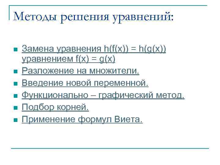Methods for solving the equations: n n n Replacing the equation h (f (x)) \u003d h (g (x)) with the equation f (x) \u003d g (x) Factorization. Introduction of a new variable. Functionally - graphic method. The selection of roots. Application of Vieta formulas.

Replacing the equation h (f (x)) \u003d h (g (x)) with the equation f (x) \u003d g (x). The method can be applied only if y \u003d h (x) is a monotonic function that takes its own value once. If the function is nonmonotonic, then root loss is possible.

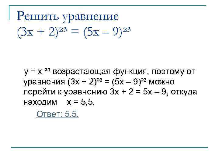Solve the equation (3 x + 2) ²³ \u003d (5 x - 9) ²³ y \u003d x ²³ is an increasing function, therefore, from the equation (3 x + 2) ²³ \u003d (5 x - 9) ²³ you can go to the equation 3 x + 2 \u003d 5 x - 9, whence we find x \u003d 5, 5. Answer: 5, 5.

Factorization. The equation f (x) g (x) h (x) \u003d 0 can be replaced by the set of equations f (x) \u003d 0; g (x) \u003d 0; h (x) \u003d 0. Having solved the equations of this set, we need to take those roots that belong to the domain of definition of the original equation, and discard the rest as extraneous.

Solve the equation x³ - 7 x + 6 \u003d 0 Representing the term 7 x in the form x + 6 x, we obtain sequentially: x³ - x - 6 x + 6 \u003d 0 x (x² - 1) - 6 (x - 1) \u003d 0 x (x - 1) (x + 1) - 6 (x - 1) \u003d 0 (x - 1) (x² + x - 6) \u003d 0 Now the problem is reduced to solving the set of equations x - 1 \u003d 0; x² + x - 6 \u003d 0. Answer: 1, 2, - 3.

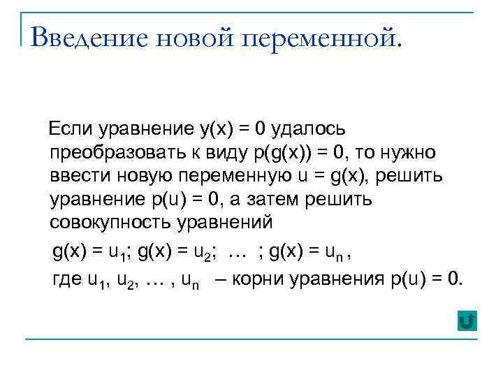Introducing a new variable. If it was possible to transform the equation y (x) \u003d 0 to the form p (g (x)) \u003d 0, then we need to introduce a new variable u \u003d g (x), solve the equation p (u) \u003d 0, and then solve the set of equations g ( x) \u003d u 1; g (x) \u003d u 2; ...; g (x) \u003d un, where u 1, u 2, ..., un are the roots of the equation p (u) \u003d 0.

Solve the equation A feature of this equation is the equality of the coefficients of its left side, equidistant from its ends. Such equations are called return equations. Since 0 is not the root of this equation, dividing by x² we get

We introduce a new variable. Then we obtain the quadratic equation. So, the root y 1 \u003d - 1 can not be considered. We will get the Answer: 2, 0, 5.

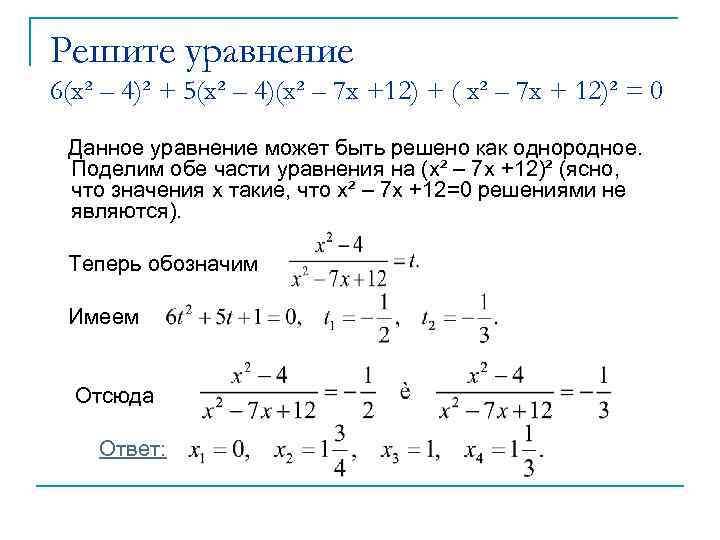Solve Equation 6 (x² - 4) ² + 5 (x² - 4) (x² - 7 x +12) + (x² - 7 x + 12) ² \u003d 0 This equation can be solved as a homogeneous one. We divide both sides of the equation by (x² - 7 x +12) ² (it is clear that the values \u200b\u200bof x are such that x² - 7 x + 12 \u003d 0 are not solutions). Now we denote We have From here the Answer:

Functionally - graphic method. If one of the functions y \u003d f (x), y \u003d g (x) increases, and the other decreases, then the equation f (x) \u003d g (x) either has no roots or has one root.

Solve the equation It is fairly obvious that x \u003d 2 is the root of the equation. Let us prove that this is the only root. We transform the equation to the form. We notice that the function increases and the function decreases. Therefore, the equation has only one root. Answer: 2.

Selection of roots n n n Theorem 1: If an integer m is a root of a polynomial with integer coefficients, then the free term of the polynomial is divided by m. Theorem 2: A reduced polynomial with integer coefficients has no fractional roots. Theorem 3: - an equation with integer Let coefficients. If the number and fraction where p and q are integers is irreducible, is the root of the equation, then p is the divisor of the free term an, and q is the divisor of the coefficient with the leading term a 0.

Bezout theorem. The remainder when dividing any polynomial by a binomial (x - a) is equal to the value of the divisible polynomial at x \u003d a. Corollaries of the Bezout theorem n n n n The difference of the same powers of two numbers is divisible without remainder by the difference of the same numbers; The difference of equal even powers of two numbers is divided without remainder both by the difference of these numbers, and by their sum; The difference of the same odd powers of two numbers is not divided by the sum of these numbers; The sum of the equal powers of two non-numbers is divided by the difference of these numbers; The sum of identical odd powers of two numbers is divided without remainder by the sum of these numbers; The sum of identical even powers of two numbers is not divided both by the difference of these numbers, and by their sum; A polynomial is completely divided by a binomial (x - a) if and only if the number a is the root of the given polynomial; The number of different roots of a non-zero polynomial is no more than its degree.

Solve the equation x³ - 5 x² - x + 21 \u003d 0 The polynomial x³ - 5 x² - x + 21 has integer coefficients. By Theorem 1, its integer roots, if any, are among the divisors of the free term: ± 1, ± 3, ± 7, ± 21. By checking, we verify that the number 3 is a root. By the corollary of Bezout's theorem, the polynomial is divided into (x - 3). Thus, x³– 5 x² - x + 21 \u003d (x - 3) (x²– 2 x - 7). Answer:

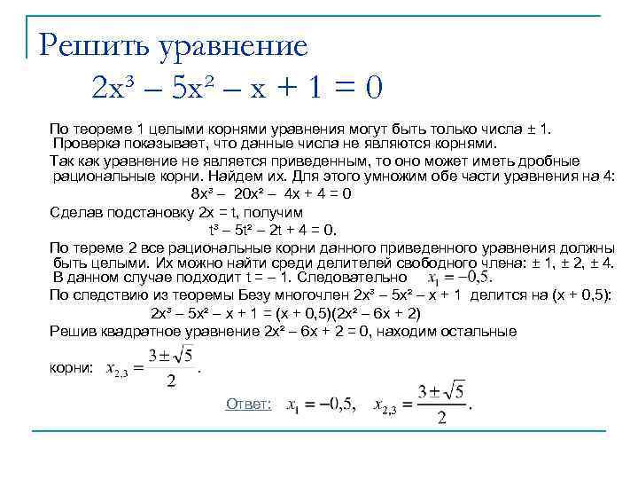Solve the equation 2 x³ - 5 x² - x + 1 \u003d 0 By Theorem 1, only the numbers ± 1 can be the whole roots of the equation. Verification shows that these numbers are not roots. Since the equation is not reduced, it can have fractional rational roots. Find them. To do this, we multiply both sides of the equation by 4: 8 x³ - 20 x² - 4 x + 4 \u003d 0 By substituting 2 x \u003d t, we obtain t³ - 5 t² - 2 t + 4 \u003d 0. By Theorem 2, all rational roots of this reduced equation must be whole. They can be found among the divisors of the free term: ± 1, ± 2, ± 4. In this case, t \u003d - 1. Therefore, by the corollary of the Bezout theorem, the polynomial 2 x³ - 5 x² - x + 1 is divided by (x + 0, 5 ): 2 x³ - 5 x² - x + 1 \u003d (x + 0, 5) (2 x² - 6 x + 2) Solving the quadratic equation 2 x² - 6 x + 2 \u003d 0, we find the remaining roots: Answer:

Solve the equation 6 x³ + x² - 11 x - 6 \u003d 0 By Theorem 3, the rational roots of this equation should be sought among the numbers Substituting them one by one in the equation, we find that they satisfy the equation. They exhaust all the roots of the equation. Answer:

Find the sum of the squares of the roots of the equation x³ + 3 x² - 7 x +1 \u003d 0 By Vieta's theorem Note that whence

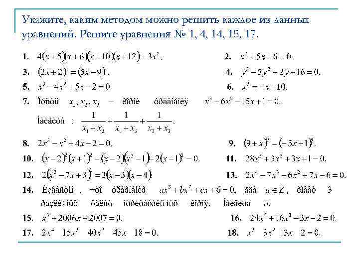Indicate by which method each of these equations can be solved. Solve equations number 1, 4, 15, 17.

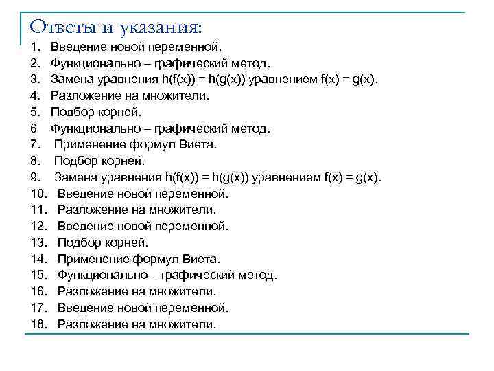Answers and instructions: 1. Introduction of a new variable. 2. Functional - graphical method. 3. Replacing the equation h (f (x)) \u003d h (g (x)) with the equation f (x) \u003d g (x). 4. Factorization. 5. The selection of roots. 6 Functional - graphical method. 7. Application of the Vieta formulas. 8. The selection of roots. 9. Replacing the equation h (f (x)) \u003d h (g (x)) with the equation f (x) \u003d g (x). 10. Introduction of a new variable. 11. Factorization. 12. Introduction of a new variable. 13. The selection of roots. 14. Application of the Vieta formulas. 15. Functionally - graphic method. 16. Factorization. 17. Introduction of a new variable. 18. Factorization.

1. Indication. Write the equation in the form 4 (x² + 17 x + 60) (x + 16 x + 60) \u003d 3 x². Divide both sides by x². Enter the variable Answer: x 1 \u003d - 8; x 2 \u003d - 7, 5. 4. Note. Add 6 y and - 6 y to the left side of the equation and write it in the form (y³ - 2 y²) + (- 3 y² + 6 y) + (- 8 y + 16) \u003d (y - 2) (y² - 3 y - 8). Answer:

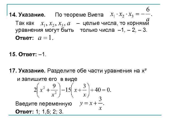14. Indication. By the Vieta theorem Since are integers, then the roots of the equation can be only numbers - 1, - 2, - 3. Answer: 15. Answer: - 1. 17. Indication. Divide both sides of the equation by x² and write it in the form Enter a variable Answer: 1; fifteen; 2; 3.

Bibliography. n n n Kolmogorov A. N. “Algebra and the beginning of analysis, 10 - 11” (M.: Education, 2003). Bashmakov M. I. "Algebra and the beginning of analysis, 10 - 11" (M.: Education, 1993). Mordkovich A. G. “Algebra and the beginning of analysis, 10–11” (M.: Mnemozina, 2003). Alimov Sh. A., Kolyagin Yu.M. et al. “Algebra and the Beginning of Analysis, 10–11” (M.: Education, 2000). Galitsky M. L., Goldman A. M., Zvavich L. I. "A collection of problems in algebra, 8 - 9" (M.: Education, 1997). Karp A. P. “A collection of problems in algebra and the principles of analysis, 10–11” (M.: Education, 1999). Sharygin I. F. "An optional course in mathematics, problem solving, 10" (M.: Education. 1989). Skopets Z. A. "Additional chapters on the course of mathematics, 10" (M.: Education, 1974). Litinsky G. I. "Lessons in Mathematics" (M.: Aslan, 1994). G. Muravin, “Equations, Inequalities, and Their Systems” (Mathematics, Appendix to the newspaper Pervoe September, No. 2, 3, 2003). Kolyagin Yu. M. “Polynomials and equations of higher degrees” (Mathematics, Appendix to the newspaper “First of September”, No. 3, 2005).

Consider solving equations with one variable of degree higher than the second.

The degree of the equation P (x) \u003d 0 is the degree of the polynomial P (x), i.e. the largest of the degrees of its members with a coefficient not equal to zero.

So, for example, the equation (x 3 - 1) 2 + x 5 \u003d x 6 - 2 has a fifth power, because after the operations of opening the brackets and bringing down similar ones, we obtain the equivalent equation x 5 - 2x 3 + 3 \u003d 0 of the fifth degree.

Recall the rules that will be needed to solve equations of degree higher than the second.

Statements about the roots of the polynomial and its divisors:

1. A polynomial of degree n has a number of roots that does not exceed number n, and roots of multiplicity m occur exactly m times.

2. An odd degree polynomial has at least one real root.

3. If α is the root of P (x), then P n (x) \u003d (x - α) · Q n - 1 (x), where Q n - 1 (x) is a polynomial of degree (n - 1).

5. The reduced polynomial with integer coefficients cannot have fractional rational roots.

6. For a polynomial of the third degree

P 3 (x) \u003d ax 3 + bx 2 + cx + d one of the two is possible: either it decomposes into the product of three binomials

P 3 (x) \u003d a (x - α) (x - β) (x - γ), or decomposes into the product of the binomial and the square trinomial P 3 (x) \u003d a (x - α) (x 2 + βx + γ )

7. Any fourth-degree polynomial decomposes into a product of two square trinomials.

9. For the polynomial P (x) to be divisible by the binomial (x - c), it is necessary and sufficient that the number with be the root of P (x) (Corollary to Bezout's theorem).

10. Vieta's theorem: If x 1, x 2, ..., x n are the real roots of the polynomial

P (x) \u003d a 0 x n + a 1 x n - 1 + ... + a n, then the following equalities hold:

x 1 + x 2 + ... + x n \u003d -a 1 / a 0,

x 1 · x 2 + x 1 · x 3 + ... + x n - 1 · x n \u003d a 2 / a 0,

x 1 · x 2 · x 3 + ... + x n - 2 · x n - 1 · x n \u003d -a 3 / a 0,

x 1 · x 2 · x 3 · x n \u003d (-1) n a n / a 0.

Solution Examples

Example 1

Find the remainder of the division of P (x) \u003d x 3 + 2/3 x 2 - 1/9 by (x - 1/3).

Decision.

By the corollary of Bezout’s theorem: “The remainder of dividing a polynomial by a binomial (x - c) is equal to the value of the polynomial in c”. We find P (1/3) \u003d 0. Therefore, the remainder is 0 and the number 1/3 is the root of the polynomial.

Answer: R \u003d 0.

Example 2

Divide the "corner" 2x 3 + 3x 2 - 2x + 3 by (x + 2). Find the remainder and the partial quotient.

Decision:

2x 3 + 3x 2 - 2x + 3 | x + 2

2x 3 + 4 x 2 2x 2 - x

X 2 - 2 x

Answer: R \u003d 3; quotient: 2x 2 - x.

Basic methods for solving equations of higher degrees

1. Introduction of a new variable

The method of introducing a new variable is already familiar with the example of biquadratic equations. It consists in the fact that to solve the equation f (x) \u003d 0, a new variable (substitution) t \u003d x n or t \u003d g (x) is introduced and f (x) is expressed in terms of t, obtaining a new equation r (t). Solving then the equation r (t), find the roots:

(t 1, t 2, ..., t n). After that, a set of n equations q (x) \u003d t 1, q (x) \u003d t 2, ..., q (x) \u003d t n is obtained, from which the roots of the original equation are found.

Example 1

(x 2 + x + 1) 2 - 3x 2 - 3x - 1 \u003d 0.

Decision:

(x 2 + x + 1) 2 - 3 (x 2 + x) - 1 \u003d 0.

(x 2 + x + 1) 2 - 3 (x 2 + x + 1) + 3 - 1 \u003d 0.

Replacement (x 2 + x + 1) \u003d t.

t 2 - 3t + 2 \u003d 0.

t 1 \u003d 2, t 2 \u003d 1. Reverse replacement:

x 2 + x + 1 \u003d 2 or x 2 + x + 1 \u003d 1;

x 2 + x - 1 \u003d 0 or x 2 + x \u003d 0;

Answer: From the first equation: x 1, 2 \u003d (-1 ± √5) / 2, from the second: 0 and -1.

2. Factorization by grouping and shorthand multiplication formulas

The basis of this method is also not new and consists in grouping the terms in such a way that each group contains a common factor. To do this, sometimes you have to apply some artificial tricks.

Example 1

x 4 - 3x 2 + 4x - 3 \u003d 0.

Decision.

Imagine - 3x 2 \u003d -2x 2 - x 2 and group:

(x 4 - 2x 2) - (x 2 - 4x + 3) \u003d 0.

(x 4 - 2x 2 +1 - 1) - (x 2 - 4x + 3 + 1 - 1) \u003d 0.

(x 2 - 1) 2 - 1 - (x - 2) 2 + 1 \u003d 0.

(x 2 - 1) 2 - (x - 2) 2 \u003d 0.

(x 2 - 1 - x + 2) (x 2 - 1 + x - 2) \u003d 0.

(x 2 - x + 1) (x 2 + x - 3) \u003d 0.

x 2 - x + 1 \u003d 0 or x 2 + x - 3 \u003d 0.

Answer: There are no roots in the first equation, from the second: x 1, 2 \u003d (-1 ± √13) / 2.

3. Factorization by the method of indefinite coefficients

Example 1

x 3 + 4x 2 + 5x + 2 \u003d 0.

Decision.

A polynomial of degree 3 can be decomposed into a product of linear and square factors.

x 3 + 4x 2 + 5x + 2 \u003d (x - a) (x 2 + bx + c),

x 3 + 4x 2 + 5x + 2 \u003d x 3 + bx 2 + cx - ax 2 - abx - ac,

x 3 + 4x 2 + 5x + 2 \u003d x 3 + (b - a) x 2 + (cx - ab) x - ac.

Having solved the system:

(b - a \u003d 4,
(c - ab \u003d 5,
(-ac \u003d 2,

(a \u003d -1,
(b \u003d 3,
(c \u003d 2, i.e.

x 3 + 4x 2 + 5x + 2 \u003d (x + 1) (x 2 + 3x + 2).

The roots of the equation (x + 1) (x 2 + 3x + 2) \u003d 0 are easily found.

Answer: -1; -2.

4. Method of root selection by senior and free coefficient

The method relies on the application of theorems:

1) Every integer root of a polynomial with integer coefficients is a divisor of the free term.

2) In order for the irreducible fraction p / q (p is an integer, q is a positive integer) to be the root of the equation with integer coefficients, it is necessary that the number p be the integer divisor of the free term and 0, and q is the natural divisor of the highest coefficient.

Example 1

6x 3 + 7x 2 - 9x + 2 \u003d 0.

Decision:

6: q \u003d 1, 2, 3, 6.

Therefore, p / q \u003d ± 1, ± 2, ± 1/2, ± 1/3, ± 2/3, ± 1/6.

Having found one root, for example - 2, we will find other roots using angle division, the method of indefinite coefficients or Horner's scheme.

Answer: -2; 1/2; 1/3.

Still have questions? Not sure how to solve the equations?
To get tutor help.
The first lesson is free!

blog.site, with full or partial copying of material, a reference to the source is required.

When solving algebraic equations, one often has to factor the polynomial. Factorizing a polynomial means representing it as a product of two or more polynomials. We use some methods of decomposing polynomials quite often: taking out a common factor, applying reduced multiplication formulas, extracting a full square, grouping. Let's consider some more methods.

Sometimes, when factoring a polynomial, the following statements are useful:

1) if a polynomial with integer coefficients has a rational root (where is an irreducible fraction, then is the divisor of the free term and the divisor of the highest coefficient:

2) If in some way we choose the root of the polynomial of degree, then the polynomial can be represented in the form where the polynomial of degree

The polynomial can be found either by dividing the polynomial into a binomial “column”, or by correspondingly grouping the terms of the polynomial and extracting a factor from them, or by the method of indefinite coefficients.

Example. Factor polynomial

Decision. Since the coefficient at x4 is 1, the rational roots of this polynomial exist, are divisors of 6, that is, they can be integers ± 1, ± 2, ± 3, ± 6. Denote this polynomial by P4 (x). Since P P4 (1) \u003d 4 and P4 (-4) \u003d 23, the numbers 1 and -1 are not the roots of the polynomial PA (x). Since P4 (2) \u003d 0, then x \u003d 2 is the root of the polynomial P4 (x), and, therefore, this polynomial is divided by the binomial x - 2. Therefore, x4 -5x3 + 7x2 -5x +6 x-2 x4 -2x3 x3 -3x2 + x-3

3x3 + 7x2 -5x +6

3x3 + 6x2 x2 - 5x + 6 x2 - 2x

Consequently, P4 (x) \u003d (x - 2) (x3 - 3x2 + x - 3). Since xz - 3x2 + x - 3 \u003d x2 (x - 3) + (x - 3) \u003d (x - 3) (x2 + 1), then x4 - 5x3 + 7x2 - 5x + 6 \u003d (x - 2) (x - 3) (x2 + 1).

Parameter Input Method

Sometimes, when factoring a polynomial, the method of introducing a parameter helps. We explain the essence of this method in the following example.

Example. x3 - (√3 + 1) x2 + 3.

Decision. Consider a polynomial with the parameter a: x3 - (a + 1) x2 + a2, which for a \u003d √3 turns into a given polynomial. We write this polynomial as a quadratic trinomial with respect to a: ar - ax2 + (x3 - x2).

Since the roots of this quadratic trinomial with respect to a are a1 \u003d x and a2 \u003d x2 - x, then the equality a2 - ax2 + (xs - x2) \u003d (a - x) (a - x2 + x) is valid. Therefore, the polynomial x3 - (√3 + 1) x2 + 3 is factorized as √3 - x and √3 - x2 + x, i.e.

x3 - (√3 + 1) x2 + 3 \u003d (x-√3) (x2-x-√3).

Method for introducing a new unknown

In some cases, by replacing the expression f (x) in the polynomial Pn (x), we can obtain a polynomial with respect to y through y, which can already be easily factorized. Then, after changing y to f (x), we obtain the factorization of the polynomial Pn (x).

Example. Factor the polynomial x (x + 1) (x + 2) (x + 3) -15.

Decision. We transform this polynomial as follows: x (x + 1) (x + 2) (x + 3) -15 \u003d [x (x + 3)] [(x + 1) (x + 2)] - 15 \u003d (x2 + 3x) (x2 + 3x + 2) - 15.

Denote x2 + 3x by y. Then we have y (y + 2) - 15 \u003d y2 + 2y - 15 \u003d y2 + 2y + 1 - 16 \u003d (y + 1) 2 - 16 \u003d (y + 1 + 4) (y + 1 - 4) \u003d ( y + 5) (y - 3).

Therefore, x (x + 1) (x + 2) (x + 3) - 15 \u003d (x2 + 3x + 5) (x2 + 3x - 3).

Example. Factor polynomial (x-4) 4+ (x + 2) 4

Decision. Denote x - 4 + x + 2 \u003d x - 1 by y.

(x - 4) 4 + (x + 2) 2 \u003d (y - 3) 4 + (y + 3) 4 \u003d y4 - 12y3 + 54y3 - 108y + 81 + y4 + 12y3 + 54y2 + 108y + 81 \u003d

2y4 + 108y2 + 162 \u003d 2 (y4 + 54y2 + 81) \u003d 2 [(yy + 27) 2 - 648] \u003d 2 (y2 + 27 - √b48) (y2 + 27 + √b48) \u003d

2 ((x-1) 2 + 27-√b48) ((x-1) 2 + 27 + √b48) \u003d 2 (x2-2x + 28--18√2) (x2-2x + 28 + 18√ 2 )

Combination of different methods

Often, when factoring a polynomial, several of the methods discussed above must be applied sequentially.

Example. Factor the polynomial x4 - 3x2 + 4x-3.

Decision. Using the grouping, we rewrite the polynomial in the form x4 - 3x2 + 4x - 3 \u003d (x4 - 2x2) - (x2 -4x + 3).

Applying the full square selection method to the first bracket, we have x4 - 3x3 + 4x - 3 \u003d (x4 - 2 · 1 · x2 + 12) - (x2 -4x + 4).

Using the full square formula, we can now write that x4 - 3x2 + 4x - 3 \u003d (x2 -1) 2 - (x - 2) 2.

Finally, applying the formula of the difference of squares, we get that x4 - 3x2 + 4x - 3 \u003d (x2 - 1 + x - 2) (x2 - 1 - x + 2) \u003d (x2 + x-3) (x2-x + 1 )

§ 2. Symmetric equations

1. Symmetric equations of the third degree

Equations of the form ax3 + bx2 + bx + a \u003d 0, and ≠ 0 (1) are called symmetric equations of the third degree. Since ax3 + bx2 + bx + a \u003d a (x3 + 1) + bx (x + 1) \u003d (x + 1) (ax2 + (b-a) x + a), then equation (1) is equivalent to the set of equations x + 1 \u003d 0 and ax2 + (b-a) x + a \u003d 0, which is not difficult to solve.

Example 1. Solve the equation

3x3 + 4x2 + 4x + 3 \u003d 0. (2)

Decision. Equation (2) is a symmetric equation of the third degree.

Since 3x3 + 4xg + 4x + 3 \u003d 3 (x3 + 1) + 4x (x + 1) \u003d (x + 1) (3x2 - 3x + 3 + 4x) \u003d (x + 1) (3x2 + x + 3) , then equation (2) is equivalent to the set of equations x + 1 \u003d 0 and 3x3 + x + 3 \u003d 0.

The solution to the first of these equations is x \u003d -1, the second equation has no solutions.

Answer: x \u003d -1.

2. Symmetric equations of the fourth degree

Equation of the form

(3) is called a symmetric equation of the fourth degree.

Since x \u003d 0 is not the root of equation (3), then, dividing both sides of equation (3) by x2, we obtain an equation equivalent to the original (3):

We rewrite equation (4) in the form:

In this equation we make a replacement, then we obtain the quadratic equation

If equation (5) has 2 roots y1 and y2, then the original equation is equivalent to the set of equations

If equation (5) has one root y0, then the original equation is equivalent to the equation

Finally, if equation (5) has no roots, then the original equation also has no roots.

Example 2. Solve the equation

Decision. This equation is a symmetric equation of the fourth degree. Since x \u003d 0 is not its root, then, dividing equation (6) by x2, we obtain the equation equivalent to it:

Having grouped the terms, we rewrite equation (7) in the form or in the form

Putting, we obtain an equation having two roots y1 \u003d 2 and y2 \u003d 3. Therefore, the original equation is equivalent to a set of equations

The solution to the first equation of this set is x1 \u003d 1, and the solution to the second is and.

Therefore, the original equation has three roots: x1, x2 and x3.

Answer: x1 \u003d 1 ,.

§3. Algebraic equations

1. The decrease in the degree of equation

Some algebraic equations by replacing a certain polynomial in them with one letter can be reduced to algebraic equations whose degree is less than the degree of the original equation and the solution of which is simpler.

Example 1. Solve the equation

Decision. We denote by, then equation (1) can be rewritten in the form The last equation has roots and Therefore, equation (1) is equivalent to the set of equations and. There is a solution to the first equation of this set and there are solutions to the second equation

The solutions of equation (1) are

Example 2. Solve the equation

Decision. Multiplying both sides of the equation by 12 and denoting by,

We get the equation Rewrite this equation in the form

(3) and denoting by rewriting equation (3) in the form The last equation has roots, and therefore we find that equation (3) is equivalent to the combination of two equations and there are solutions to this set of equations, i.e., equation (2) is equivalent to the combination of equations and ( four)

The solutions of (4) are and, they are the solutions of equation (2).

2. Equations of the form

The equation

(5) where are given numbers, can be reduced to a biquadratic equation by replacing the unknown, i.e., replacing

Example 3. Solve the equation

Decision. Denote by, t. e. make a change of variables or Then equation (6) can be rewritten in the form or, using the formula, in the form

Since the roots of the quadratic equation are, and then the solutions of equation (7) are the solutions of the set of equations and. This set of equations has two solutions and, therefore, the solutions of equation (6) are and

3. Equations of the form

The equation

(8) where the numbers α, β, γ, δ, and Α are such that α

Example 4. Solve the equation

Decision. We replace the unknowns, i.e., y \u003d x + 3 or x \u003d y - 3. Then equation (9) can be rewritten in the form

(y-2) (y-1) (y + 1) (y + 2) \u003d 10, i.e., in the form

(y2-4) (y2-1) \u003d 10 (10)

Biquadratic equation (10) has two roots. Therefore, equation (9) also has two roots:

4. Equations of the form

Equation, (11)

Where, has no root x \u003d 0, therefore, dividing equation (11) by x2, we obtain the equation equivalent to it

Which, after replacing the unknown, will be rewritten in the form of a quadratic equation, the solution of which is not difficult.

Example 5. Solve the equation

Decision. Since h \u003d 0 is not the root of equation (12), dividing it by x2, we obtain the equation equivalent to it

Making the substitution unknown, we obtain the equation (y + 1) (y + 2) \u003d 2, which has two roots: y1 \u003d 0 and y1 \u003d -3. Therefore, the original equation (12) is equivalent to the set of equations

This set has two roots: x1 \u003d -1 and x2 \u003d -2.

Answer: x1 \u003d -1, x2 \u003d -2.

Comment. Equation of the form

In which, one can always bring to the form (11) and, moreover, considering α\u003e 0 and λ\u003e 0 to the form.

5. Equations of the form

The equation

, (13) where the numbers, α, β, γ, δ, and Α are such that αβ \u003d γδ ≠ 0, we can rewrite it by multiplying the first bracket with the second and the third with the fourth, in the form, i.e., equation (13) now written in the form (11), and its solution can be carried out in the same way as the solution of equation (11).

Example 6. Solve the equation

Decision. Equation (14) has the form (13), so we rewrite it in the form

Since x \u003d 0 is not a solution to this equation, dividing both its parts by x2, we obtain an equivalent initial equation. Making a change of variables, we obtain a quadratic equation, the solution of which is and. Therefore, the original equation (14) is equivalent to the set of equations and.

The solution to the first equation of this population is

The second equation of this set of solutions has no. So, the original equation has roots x1 and x2.

6. Equations of the form

The equation

(15) where the numbers a, b, c, q, A are such that, does not have a root x \u003d 0, therefore, dividing equation (15) by x2. we obtain an equation equivalent to it, which, after replacing the unknown, will be rewritten in the form of a quadratic equation, the solution of which is not difficult.

Example 7. The solution of the equation

Decision. Since x \u003d 0 is not the root of equation (16), then, dividing both its parts by x2, we obtain the equation

, (17) equivalent to equation (16). Having made the replacement unknown, we rewrite equation (17) in the form

Quadratic equation (18) has 2 roots: y1 \u003d 1 and y2 \u003d -1. Therefore, equation (17) is equivalent to a combination of equations and (19)

The set of equations (19) has 4 roots:,.

They will be the roots of equation (16).

§four. Rational equations

Equations of the form \u003d 0, where H (x) and Q (x) are polynomials, are called rational.

Having found the roots of the equation H (x) \u003d 0, then we need to check which of them are not the roots of the equation Q (x) \u003d 0. These roots and only they will be solutions to the equation.

Consider some methods for solving equations of the form \u003d 0.

1. Equations of the form

The equation

(1) under certain conditions on numbers, it can be solved as follows. Grouping the terms of equation (1) in two and summing each pair, you need to get polynomials of the first or zero degree in the numerator, differing only in numerical factors, and in the denominators - trinomials with the same two terms containing x, then after changing the variables, the equation will either have also the form (1), but with a smaller number of terms, either will be equivalent to a combination of two equations, one of which will be the first degree, and the second will be an equation of the form (1), but with a smaller number of terms.

Example. Solve the equation

Decision. Grouping on the left side of equation (2) the first term with the last, and the second with the penultimate, we rewrite equation (2) in the form

Summing up the terms in each bracket, we rewrite equation (3) in the form

Since there is no solution to equation (4), dividing this equation by, we obtain the equation

, (5) equivalent to equation (4). We make a replacement for the unknown, then equation (5) can be rewritten in the form

Thus, the solution of equation (2) with five terms on the left side is reduced to the solution of equation (6) of the same form, but with three terms on the left side. Summing up all the terms on the left side of equation (6), we rewrite it in the form

The solutions to the equation are and. None of these numbers vanish the denominator of the rational function on the left side of equation (7). Therefore, equation (7) has these two roots, and therefore, the original equation (2) is equivalent to the set of equations

The solutions to the first equation of this set are

The solutions of the second equation from this set are

Therefore, the original equation has roots

2. Equations of the form

The equation

(8) under certain conditions on numbers, one can solve this way: it is necessary to select the integer part in each of the fractions of the equation, i.e., replace equation (8) with equation

Reduce it to the form (1) and then solve it by the method described in the previous paragraph.

Example. Solve the equation

Decision. We write equation (9) in the form or in the form

Summing up the terms in brackets, we rewrite equation (10) in the form

Making a replacement for the unknown, we rewrite equation (11) in the form

Summing up the terms on the left side of equation (12), we rewrite it in the form

It is easy to see that equation (13) has two roots: and. Therefore, the original equation (9) has four roots:

3) Equations of the form.

An equation of the form (14) under certain conditions on numbers can be solved as follows: by expanding (if it is, of course, possible) each of the fractions on the left side of equation (14) into a sum of simple fractions

Reduce equation (14) to form (1), then, after conveniently rearranging the terms of the resulting equation, solve it by the method described in paragraph 1).

Example. Solve the equation

Decision. Since and, then, multiplying the numerator of each fraction in equation (15) by 2 and noting that equation (15) can be written as

Equation (16) has the form (7). Regrouping the terms in this equation, we rewrite it in the form or in the form

Equation (17) is equivalent to a combination of equations and

To solve the second equation of the set (18), we make the replacement of the unknown Then it will be rewritten in the form or in the form

Summing up all the terms on the left side of equation (19), rewrite it as

Since the equation has no roots, then equation (20) also does not have them.

The first equation of the population (18) has a single root Since this root is included in the ODZ of the second equation of the population (18), it is the only root of the population (18), and hence the original equation.

4. Equations of the form

The equation

(21) under certain conditions on the numbers and A, after presenting each term on the left side in the form, it can be reduced to the form (1).

Example. Solve the equation

Decision. We rewrite equation (22) in the form or in the form

Thus, equation (23) is reduced to the form (1). Now, grouping the first term with the last, and the second with the third, we rewrite equation (23) in the form

This equation is equivalent to the set of equations and. (24)

The last equation of the set (24) can be rewritten in the form

There are solutions to this equation, and since it is included in the ODZ of the second equation of the set (30), then the set (24) has three roots :. All of them are solutions to the original equation.

5. Equations of the form.

Equation of the form (25)

Under certain conditions, by replacing the unknown, the numbers can be reduced to an equation of the form

Example. Solve the equation

Decision. Since it is not a solution to equation (26), then dividing the numerator and denominator of each fraction on the left side by, we rewrite it in the form

After changing the variables, we rewrite equation (27) in the form

Solving equation (28) is and. Therefore, equation (27) is equivalent to the set of equations and. (29)

The text of the work is posted without images and formulas.
The full version of the work is available in the tab "Files of work" in PDF format

Introduction

Solving algebraic equations of higher degrees with one unknown is one of the most difficult and oldest mathematical problems. The most outstanding mathematicians of antiquity were engaged in these tasks.

The solution of equations of the nth degree is an important task for modern mathematics. The interest in them is quite large, since these equations are closely related to the search for the roots of equations that are not considered by the school curriculum in mathematics.

Problem: the lack of skills in solving equations of higher degrees in various ways among students prevents them from successfully preparing for final certification in mathematics and mathematical olympiads, teaching in a specialized mathematical class.

The listed facts identified relevance our work "Solving equations of higher degrees."

Possession of the simplest methods for solving equations of the nth degree reduces the time to complete the task, on which the result of work and the quality of the learning process depend.

Objective: the study of known methods for solving equations of higher degrees and identifying the most accessible of them for practical use.

Based on the goal, the following tasks:

To study the literature and Internet resources on this topic;

Get acquainted with historical facts related to this topic;

Describe the various ways of solving equations of higher degrees

compare the degree of difficulty of each of them;

To acquaint classmates with methods for solving equations of higher degrees;

Create a selection of equations for the practical application of each of the considered methods.

Object of study - equations of higher degrees with one variable.

Subject of study - methods for solving equations of higher degrees.

Hypothesis:a common method and a single algorithm that allows finding solutions of equations of the nth degree in a finite number of steps does not exist.

Research Methods:

- bibliographic method (analysis of literature on the research topic)

- classification method;

- qualitative analysis method.

Theoretical significanceresearch consists in systematizing methods for solving equations of higher degrees and a description of their algorithms.

Practical significance - Presented material on this topic and the development of a textbook for students on this topic.

1. EQUATIONS OF THE HIGHEST DEGREES

1.1 the Concept of the equation of the n-th degree

Definition 1.An equation of the nth degree is an equation of the form

a 0 xⁿ + a 1 xn -1 + a 2 xⁿ - ² + ... + an -1 x + an \u003d 0, where the coefficients a 0, a 1, a 2…, an -1, an- any real numbers, moreover , a 0 ≠ 0 .

Polynomial a 0 xⁿ + a 1 xn -1 + a 2 xⁿ - ² + ... + an -1 x + an is called an nth degree polynomial. Odds are distinguished by name: a 0 - senior coefficient; an is a free member.

Definition 2. The solutions or roots for this equation are all variable values xwhich convert this equation to true numerical equality or, in which the polynomial a 0 xⁿ + a 1 xn -1 + a 2 xⁿ - ² + ... + an -1 x + an vanishes. This variable value xalso called the root of the polynomial. To solve the equation means to find all its roots or to establish that they are not.

If a 0 \u003d 1, then such an equation is called a reduced integer rational equation n th degrees.

For equations of the third and fourth degree, there are Cardano and Ferrari formulas that express the roots of these equations through radicals. It turned out that in practice they are rarely used. Thus, if n ≥ 3, and the polynomial coefficients are arbitrary real numbers, then the search for the roots of the equation is not an easy task. Nevertheless, in many special cases this problem is solved to the end. Let us dwell on some of them.

1.2 Historical facts of solving equations of higher degrees

A universal formula for finding the roots of an algebraic equation nth no degree. Many, of course, had the tempting idea to find formulas for any degree n that express the roots of the equation in terms of its coefficients, that is, solve the equation in radicals.

Only in the 16th century did Italian mathematicians advance further by finding formulas for n \u003d 3 and n \u003d 4. At the same time, Scipio, Dahl, Ferro and his students Fiori and Tartaglia dealt with the general solution of equations of the 3rd degree.

In 1545, the book of the Italian mathematician D. Cardano, “The Great Art, or the Rules of Algebra,” was published, where, along with other questions of algebra, general methods for solving cubic equations are considered, as well as a method for solving equations of the 4th degree, discovered by his student L. Ferrari.

A complete statement of the questions connected with the solution of equations of the 3rd and 4th degrees was given by F. Viet.

In the 20s of the 19th century, the Norwegian mathematician N. Abel proved that the roots of equations of the fifth degree cannot be expressed through radicals.

The study revealed that modern science knows many ways to solve equations of the nth degree.

The search for methods for solving equations of higher degrees that cannot be solved by the methods considered in the school curriculum resulted in methods based on the application of the Vieta theorem (for equations of degree n\u003e 2), Bezout's theorem, Horner's scheme, as well as the Cardano and Ferrari formula for solving cubic equations and equations of the fourth degree.

The paper presents methods for solving equations and their types, which have become a discovery for us. These include - the method of uncertain coefficients, the selection of the full degree, symmetric equations.

2. SOLUTION OF THE WHOLE EQUATIONS OF THE HIGHEST DEGREES WITH WHOLE COEFFICIENTS

2.1 Solution of equations of the 3rd degree. Formula D. Cardano

We consider equations of the form x 3 + px + q \u003d 0.We transform the equation of the general form to the form: x 3 + px 2 + qx + r \u003d 0. We write the formula for the cube of the sum; Add to the original equality and replace it with y. We get the equation: y 3 + (q -) (y -) + (r - \u003d 0. After the transformations, we have: y 2 + py + q \u003d 0. Now, again, write the formula for the cube of the sum:

(a + b) 3 \u003d a 3 + 3a 2 b + 3ab 2 + b 3 \u003d a 3 + b 3 + 3ab (a + b), replace ( a + b)on xwe get the equation x 3 - 3abx - (a 3 + b 3) = 0. Now it is clear that the original equation is equivalent to the system: and Solving the system, we obtain:

We got a formula for solving the reduced equation of the 3rd degree. She bears the name of the Italian mathematician Cardano.

Consider an example. Solve the equation:.

We have r \u003d 15 and q \u003d 124, then using the Cardano formula, we calculate the root of the equation

Conclusion: this formula is good, but not suitable for solving all cubic equations. However, it is bulky. Therefore, in practice it is rarely used.

But those who master this formula can use it when solving equations of the third degree on the exam.

2.2 Vieta Theorem

From a course in mathematics we know this theorem for a quadratic equation, but few people know that it is used to solve equations of higher degrees.

Consider the equation:

factor the left side of the equation, divide by ≠ 0.

We transform the right side of the equation to the form

; it follows that we can write the following equalities into the system:

The formulas deduced by Viet for quadratic equations and demonstrated by us for equations of degree 3 are also true for polynomials of higher degrees.

We solve the cubic equation:

Conclusion: this method is universal and easy enough for students to understand, since they know the Vieta theorem from the school curriculum for n = 2. At the same time, in order to find the roots of equations using this theorem, one must have good computational skills.

2.3 Bezout theorem

This theorem is named after the French mathematician of the 18th century J. Bezout.

Theorem.If the equation a 0 xⁿ + a 1 xn -1 + a 2 xⁿ - ² + ... + an -1 x + an \u003d 0, in which all the coefficients are integers, and the free term is non-zero, has an integer root, then this root is a divisor of the free term.

Considering that the polynomial of the nth power is on the left side of the equation, the theorem has a different interpretation.

Theorem. When dividing a polynomial of degree n with respect to x on the binomial x - a the remainder is the value of the dividend for x \u003d a. (letter a can mean any real or imaginary number, i.e. any complex number).

Evidence: let be f (x) denotes an arbitrary polynomial of degree n with respect to the variable x and let it be divided by the binomial ( x-a) it turned out in private q (x), and the remainder R. It's obvious that q (x) there will be some polynomial (n - 1st) degree relative x, and the remainder R will be a constant value, i.e. independent of x.

If the remainder R was a polynomial of the first degree with respect to x, this would mean that the division was not performed. So, R from x does not depend. By the definition of division, we obtain the identity: f (x) \u003d (x-a) q (x) + R.

Equality is valid for any value of x; therefore, it is also valid for x \u003d awe get: f (a) \u003d (a-a) q (a) + R. Symbol f (a) denotes the value of the polynomial f (x) at x \u003d a, q (a) denotes a value q (x) at x \u003d a.The remainder R stayed the way he used to be since R from x does not depend. Composition ( x-a) q (a) \u003d 0, since the factor ( x-a) \u003d 0, and the multiplier q (a) there is a certain number. Therefore, from the equality we get: f (a) \u003d R,t.d.

Example 1Find the remainder of a polynomial division x 3 - 3x 2 + 6x-5 on the binomial

x-2. By the Bezout theorem : R \u003d f(2) = 23-322 + 62 -5 \u003d 3. Answer: R \u003d3.

We note that Bezout's theorem is not so important in itself as it is by its consequences. (Annex 1)

Let us dwell on some methods of applying Bezout's theorem to solving practical problems. It should be noted that when solving equations using the Bezout theorem, it is necessary:

Find all integer divisors of a free member;

From these divisors find at least one root of the equation;

The left side of the equation is divided into (Ha);

Write the product of the divisor and the quotient on the left side of the equation;

Solve the resulting equation.

Consider the example of solving the equation x 3 + 4x 2 + x -6 = 0 .

Solution: find the free term divisors ± 1 ; ± 2; ± 3; ± 6. We calculate the values \u200b\u200bfor x \u003d1, 1 3 + 41 2 + 1-6 \u003d 0. Divide the left side of the equation by ( x-1). The division is performed by the “corner”, we get:

Conclusion: Bezout's theorem is one of the methods that we consider in our work that is studied in the program of elective classes. It is difficult to understand, because in order to own it, you need to know all the consequences of it, but Bezu’s theorem is one of the main assistants to students on the exam.

2.4 Horner Scheme

To divide a polynomial into a binomial x-α you can use a special simple technique invented by English mathematicians of the XVII century, later called Horner's scheme. In addition to finding the roots of the equations, according to Horner's scheme, one can more easily calculate their values. To do this, substitute the value of the variable in the polynomial Pn (x) \u003d a 0 xn + a 1 x n-1 + a 2 xⁿ - ² + ... ++ an -1 x + an (one)

Consider the division of polynomial (1) by the binomial x-α.

Express the coefficients of the partial quotient b 0 xⁿ - ¹+ b 1 xⁿ - ²+ b 2 xⁿ - ³+…+ bn -1 and the remainder r through the coefficients of the polynomial Pn ( x) and number α. b 0 \u003d a 0 , b 1 = α b 0 + a 1 , b 2 = α b 1 + a 2 …, bn -1 =

= α bn -2 + an -1 = α bn -1 + an .

Horner's calculations are presented in the form of the following table:

	but 0	a 1	a 2 ,
	b 0 \u003d a 0	b 1 = α b 0 + a 1	b 2 = α b 1 + a 2		r \u003d αb n-1 + an

Insofar as r \u003d Pn (α), then α is the root of the equation. In order to check whether α is a multiple root, the Horner scheme can already be applied to the quotient b 0 x +b 1 x + ... +bn -1 according to the table. If in the column under bn -1 it turns out again 0, which means that α is a multiple root.

Consider an example: solve the equation x 3 + 4x 2 + x -6 = 0.

We apply to the left side of the equation the factorization of the polynomial on the left side of the equation, the Horner scheme.

Solution: find the free term divisors ± 1; ± 2; ±3; ± 6.


				6 ∙ 1 + (-6) = 0

The coefficients of the quotient are the numbers 1, 5, 6, and the remainder is r \u003d 0.

Means x 3 + 4x 2 + x - 6 = (x - 1) (x 2 + 5x + 6) = 0.

From here: x - 1 \u003d 0 or x 2 + 5x + 6 = 0.

x = 1, x 1 = -2; x 2 = -3. Answer:1,- 2, - 3.

Conclusion: thus, on one equation, we showed the application of two different methods of factoring polynomials. In our opinion, the Horner scheme is the most practical and economical.

2.5 Solution of equations of the 4th degree. Ferrari Method

Pupil Cardano Louis Ferrari discovered a way to solve the equation of the 4th degree. The Ferrari method consists of two stages.

Stage I: equations of the form are represented as the product of two square trinomials this follows from the fact that the equation is of the 3rd degree and at least one solution.

Stage II: the resulting equations are solved using factorization, however, in order to find the required factorization, it is necessary to solve cubic equations.

The idea is to represent the equations in the form A 2 \u003d B 2, where A \u003d x 2 + s

B-linear function of x. Then it remains to solve the equations A \u003d ± B.

For clarity, consider the equation: We isolate the 4th degree, we get: For any dthe expression will be a full square. Add to both sides of the equation we get

On the left side is a full square, you can pick up dso that the right-hand side of (2) becomes a full square. Imagine that we have achieved this. Then our equation looks like this:

Finding the root afterwards will not be difficult. To choose the right d it is necessary that the discriminant of the right-hand side of (3) becomes zero, i.e.

So, to find d, it is necessary to solve this equation of the 3rd degree. Such an auxiliary equation is called resolvent.

We easily find the whole root of the resolvent: d \u003d1

Substituting the equation in (1), we obtain

Conclusion: the Ferrari method is universal, but complex and cumbersome. At the same time, if the solution algorithm is clear, then equations of the 4th degree can be solved by this method.

2.6 Method of uncertain coefficients

The success of solving the 4th degree equation by the Ferrari method depends on whether we solved the resolvent — the 3rd degree equation, which, as we know, is not always successful.

The essence of the method of uncertain coefficients is that the form of the factors into which the given polynomial is decomposed is guessed, and the coefficients of these factors (also polynomials) are determined by multiplying the factors and equating the coefficients for the same degrees of the variable.

Example: solve the equation:

Suppose that the left side of our equation can be decomposed into two square trinomials with integer coefficients such that the identity

Obviously, the coefficients in front of them must be equal to 1, and the free terms in one + 1, the other has 1.

The coefficients facing x. Denote them by but and and to determine them, we multiply both trinomials of the right side of the equation.

As a result, we get:

Equating the coefficients at the same degrees xon the left and right sides of equality (1), we obtain a system for finding and

Having solved this system, we will have

So, our equation is equivalent to the equation

Having solved it, we obtain the following roots:.

The method of uncertain coefficients is based on the following statements: any fourth-degree polynomial in the equation can be decomposed into the product of two second-degree polynomials; two polynomials are identically equal if and only if their coefficients are equal at equal degrees x

2.7 Symmetric equations

DefinitionAn equation of the form is called symmetric if the first coefficients in the equation on the left are equal to the first coefficients on the right.

We see that the first coefficients on the left are equal to the first coefficients on the right.

If such an equation has an odd degree, then it has a root x= - 1. Next, we can lower the degree of the equation by dividing it by ( x +one). It turns out that when dividing the symmetric equation by ( x +1) a symmetric equation of even degree is obtained. The proof of the symmetry of the coefficients is presented below. (Appendix 6) Our task is to learn how to solve symmetric equations of even degree.

For example: (1)

We solve equation (1), divide by x 2 (medium grade) \u003d 0.

We group the terms with symmetric

) + 3(x +. We denote at= x +, square both sides, hence \u003d at 2 So 2 ( at 2 or 2 at 2 + 3 solving the equation, we get at = , at \u003d 3. Next, we return to the replacement x + \u003d and x + \u003d 3. We get the equations and the first has no solution, and the second has two roots. Answer:.

Conclusion: this type of equation is not common, but if you come across it, you can solve it easily and simply without resorting to cumbersome calculations.

2.8 Allocation of the full degree

Consider the equation.

The left part is a cube of the sum (x + 1), i.e.

We extract the root of the third degree from both parts:, then we obtain

Where is the only root.

RESEARCH RESULTS

Based on the results of the work, we came to the following conclusions:

Thanks to the theory studied, we became acquainted with various methods for solving entire equations of higher degrees;

Formula D. Cardano is difficult to apply and makes it more likely to make mistakes in the calculation;

- the method of L. Ferrari allows us to reduce the solution of the equation of the fourth degree to cubic;

- Bezout's theorem can be applied both to cubic equations and to equations of the fourth degree; it is more understandable and visual in application to solving equations;

Horner's scheme helps to significantly reduce and simplify calculations in solving equations. In addition to finding the roots, according to Horner's scheme, one can more simply calculate the values \u200b\u200bof the polynomials on the left side of the equation;

Of particular interest were the solutions of equations by the method of indefinite coefficients, the solution of symmetric equations.

In the course of research, it was found that with the simplest methods for solving equations the highest degree students get acquainted in the elective class, starting from the 9th or 10th grade, as well as in special courses of visiting mathematical schools. This fact was established as a result of a survey of mathematics teachers at MBOU “Secondary School No. 9” and students who show an increased interest in the subject “mathematics”.

The most popular methods for solving equations of higher degrees that are encountered in solving olympiad, competitive problems and as a result of students preparing for exams are methods based on the application of Bezout's theorem, Horner's scheme, and the introduction of a new variable.

Demonstration of research results, i.e. methods of solving equations that are not studied in the school curriculum in mathematics, interested classmates.

Conclusion

Having studied the educational and scientific literature, Internet resources in youth educational forums